Enumeration of Geometric Configurations on a Convex Polygon
Marc Noy
Departament de Matemàtica Aplicada II, Universitat Politècnica de Catalunya
Algorithms Seminar
December 16, 1999
[summary by Michel Nguyen-The]
A properly typeset version of this document is available in
postscript and in
pdf.
If some fonts do not look right on your screen, this might be
fixed by configuring your browser (see the documentation here).
Abstract
We survey recent work on the enumeration of non-crossing
configurations on the set of vertices of a convex polygon, such as
triangulations, trees, and forests. Exact formulæ and limit laws
are determined for several parameters of interest. In the second part
of the talk we present results on the enumeration of chord diagrams
(pairings of 2n vertices of a convex polygon by means of n
disjoint pairs). We present limit laws for the number of components,
the size of the largest component and the number of crossings. The
use of generating functions and of a variation of Levy's continuity
theorem for characteristic functions enable us to establish that most
of the limit laws presented here are Gaussian. (Joint work by Marc
Noy with Philippe Flajolet and others.)
1 Analytic Combinatorics of Non-crossing
Configurations [3]
1.1 Connected graphs and general graphs
Let Pn={v1,...,vn} be a fixed set of points in the plane,
conventionally ordered counter-clockwise, that are vertices of a
regular n-gon K. Define a non-crossing graph as a graph
with vertex set Pn whose edges are straight line segments that do
not cross. A graph is connected if any two vertices can be
joined by a path. Parameters of interest are the number of edges of
connected graphs and general graphs, and the number of components of
general graphs.
-7pt
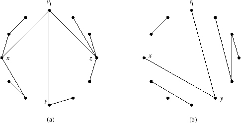
Figure 1: (a) A connected non-crossing graph; (b) an arbitrary
non-crossing graph.
1.2 Trees and forests
A (general) tree is a connected acyclic graph and the number
of edges in a tree is one less than the number of vertices. The study
of trees becomes easier with the introduction of
butterflies [3], defined to be ordered pairs of trees
with a common vertex; a tree appears to be a sequence of butterflies
attached to a root. A forest is an acyclic graph, in other
words a graph whose components are trees.
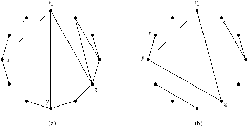
Figure 2: (a) A tree; (b) a forest.
1.3 Triangulations
A triangulation [7] is a set Tn of
n-3 non-crossing diagonals vivj which partitions K into n-2
triangles. As each triangle corresponds to an internal node of a
binary tree (see the generating function of exercise 7.22
of [6]) via a classical bijection due to
Euler [11], the number T^n of triangulations is
given by the (n-2)-th Catalan number
T^n=Cn-2=()/(n-1). Let di denote the
degree of the vertex vi (i.e., the number of diagonals
incident with vi) and ||vivj||=min(|i-j|,n-|i-j|)
the length of a diagonal vivj. Define [2]:
Dn(t)=max |
{ |
di|i=0,...,n-1 |
} |
, |
the maximal degree of the vertices, and
ln(t)=max |
{ |
||vivj|||vivjÎ Tn |
} |
, |
the length of the longest diagonal in the triangulation.
Those features are of interest for a triangulation t because they
convey information about the corresponding tree b(t):
Dn(t) measures the
external-node separation of b(t), i.e.,
the maximal distance between successive external nodes;
ln(t) measures its nearly half measure, i.e., the
size of the largest subtree with not more than half the external
nodes.
Using combinatorial bijections and probability
lemmas [2], we find:
E[Dn]~log2n, and E[ln]~a n,
where
a= |
|
+ |
|
-
|
|
~0.4654.
|
Let an ear of a triangulation t be a triangle sharing
two sides with the polygon, and en the number of ears of a
triangulation. Let us view triangulations as binary trees and ears as
leaves (internal node whose children are external nodes [11])
or roots with at least one child that is an external node, and let
B^ enumerate binary trees by size and number of leaves and
T^ enumerate triangulations by size and number of
ears.1 These generating series
satisfy [5]
z2 |
|
(z,w)= |
( |
1+2z(w-1) |
) |
|
(z,w),
where |
|
|
(z,w)=z |
æ ç ç è |
w+2 |
|
(z,w)+
|
|
(z,w)2 |
ö ÷ ÷ ø |
,
|
leading to Var[en]~(n)1/2/4 and a Gaussian limit law
(see §1.5 below). The expectation
was already known from a combinatorial manipulation of Catalan numbers
described in [7].
1.4 Generating functions
The combinatorial objects and parameters above, except for extremal
ones, lead to univariate and bivariate
generating functions, given in Table 1 below.
Configuration |
Generating function equation |
|
Connected graphs |
C3+C2-3zC+2z2=0 |
-----, edges |
wC3+wC2-(1+2w)zC+(1+w)z2=0 |
Graphs |
G2+(2z2-3z-2)G+3z+1=0 |
-----, edges |
wG2+((1+w)z2-(1+2w)z-2w)G+w+(1+2w)z=0 |
-----, components |
G3+(2w3z2-3w2z+w-3)G2+(3w2z-2w+3)G+w-1=0 |
Trees |
T3-zT+z2=0 |
-----, leaves |
T3+(z2w-z2-z)T+z2=0 |
Forests |
F3+(z2-z-3)F2+(z+3)F-1=0 |
-----, components |
F3+(w3z2-w2z-3)F2+(w3z+3)F-1=0 |
Triangulations |
z4T^2+(2z2-z)T^+1=0 |
-----, ears |
z4T^2+(1+2z(w-1))(2z2-z)
T^+w(1+2z(w-1))2=0 |
-1.5pt
Table 1: Generating function equations (z and w mark vertices and
the secondary parameter).
A few tricks enable one to make Lagrange inversion applicable and to
derive exact formulæ---sometimes involving summations---for all
coefficients. For example, the change of variable T=z+zy followed
by Lagrange's formula yields:
Finding Cn,k goes through a parameterization of the functional
equation of C. To get the coefficients T^, we use the
equality T^n,k=B^n+2,k-1+2B^n+1,k
-2B^n+1,k deduced from
z2T^(z,w)=(1+2z(w-1))B^(z,w).
1.5 Asymptotics
All of the univariate generating functions above, and a few others
(dissections and partitions of convex polygons) not presented in the
talk but available in [3], have a unique dominant
singularity r in (0,1), and can be written
f(z)=c0+c1 |
æ ç ç è |
1- |
|
ö ÷ ÷ ø |
|
+O |
æ ç ç è |
1- |
|
ö ÷ ÷ ø |
,
entailing
[zn]f(z)= |
|
|
æ ç ç è |
1+O |
æ ç ç è |
|
ö ÷ ÷ ø |
ö ÷ ÷ ø |
.
|
For example the numbers Tn and Fn of respectively general trees
and forests satisfy
Tn~(27/4)n=6.75n and Fn~8.2246n,
whence Tn=o(Fn).
The numbers Cn and Gn of respectively connected and general
graphs satisfy
Cn~ |
æ ç ç è |
|
- |
|
ö ÷ ÷ ø |
~10.39n
and
Gn~ |
|
(99(2)1/2-140)1/2×
|
2n(3+2+(2)1/2)n |
|
(p)1/2n3/2 |
|
~11.65n,
|
entailing Cn/Gn®0 when n®¥.
The bivariate generating function seen before admits the form
f(z,w)=c0(w)+c1(w) |
æ ç ç è |
1- |
|
ö ÷ ÷ ø |
|
+O |
æ ç ç è |
1- |
|
ö ÷ ÷ ø |
;
|
this leads to
fn(w)=g(w) |
æ ç ç è |
|
ö ÷ ÷ ø |
|
æ ç ç è |
1+O |
æ ç ç è |
|
ö ÷ ÷ ø |
ö ÷ ÷ ø |
, or
|
|
= |
|
æ ç ç è |
|
ö ÷ ÷ ø |
|
æ ç ç è |
1+O |
æ ç ç è |
|
ö ÷ ÷ ø |
ö ÷ ÷ ø |
.
|
From the Quasi-Powers theorem [5, 8], which is a
consequence of Levy's continuity theorem for characteristic functions,
one deduces that fn is asymptotically normal. The mean µn and
variance sn satisfy µn~k n and
sn2~l n for algebraic numbers k
and l.
For instance, for the distribution of the number of edges in the space
of connected graphs of given size, we have
k=(1+(3)1/2)/2~1.366.
2 Analytics Combinatorics of Chord Diagrams [4]
2.1 Definitions
Take 2n points on a circle, labelled 1, 2, ..., 2n, and join them
in disjoint pairs by n chords. The resulting configuration is called
a chord diagram. A diagram is connected if no set of
chords can be separated from the remaining chords by a line. A
component is a maximal connected subdiagram.
2.2 Components
2.2.1 Number of components
Let C(z)=ån³0Cnzn be the generating function of
connected diagrams of size n. The bivariate generating function
I(z,w)=ån,k³0In,kwkzn of diagrams of size n and
k components satisfies I(z,w)=1+wC(zI(z,w)2).
We have the following result:
Theorem 1
Let Xn be the number of components in a random diagram of size n.
-
For k³1, one has
P[Xn=k]=
e-1/(k-1)!(1+o(1)), n®¥.
- The mean µn and the variance sn
of the distribution satisfy
µn~2 and
sn2~1 as n®¥.
Proof.[Sketch of proof]
The proof of the first point makes use of ``monoliths,'' or
``monolithic diagrams,'' where a diagram is said to be monolithic if:
(i) it consists solely of the connected component that contains 1
(called the root component) and of isolated edges; (ii) for
any two such isolated edges (a,b) and (c,d), one never has
a<c<d<b or c<a<b<d (in other words, two isolated chords are never
in a dominance relation).
The ordinary generating function of monoliths reads
M(z)=C(z/(1-z)2), and according to Stein and
Everett [12] Cn/In=e-1+o(1), so one can deduce the
relation Mn~ In, i.e., that almost every diagram is a monolith.
The number Mn,k of monoliths of size n with k components is
given by
As to the second point, using 2zC(z)C'(z)=C(z)2+C(z)-z, which is
deduced from
and
C1=1 [9, 13], one finds
µn= |
|
(z,w) |
½ ½ ½ ½ |
|
= |
|
|
( |
I(z)+h(z)-2 |
) |
, where h(z)=I(z)-1.
|
Hence, letting gn=hn/In, one obtains
gn=1- |
|
gk |
|
|
-1
=1- |
|
+ |
|
+O(n-3),
|
and
µn=In+1+hn+1/In=2n+1/n+1+O(n-1)~2.
Similar computations yield the variance.
2.2.2 Largest connected component
Theorem 2
Let Ln be the size of the largest connected component in a random
diagram of size n. Then, as n®¥, the mean µn
and the variance sn of the distribution of Ln are
E[Ln]=n-1+o(1), Var[Ln]=1+o(1),
and for any fixed k³1, one has
P[n-Ln=k]=e-1/k!(1+o(1)).
In other words, thre random variable n-Ln follows a Poisson law
of parameter 1.
The proof relies on the analysis of the largest component in a
monolith, namely, the root component with probability 1-o(1), the
other components being only edges. The number Mn,k of monoliths
of size n with root component of size n-k is given by:
2.3 Crossings
Let k denote the number of chord crossings in a chord diagram,
and let In be the set of all diagrams of size n. Flajolet
and Noy proved the following result:
Theorem 3
Let Xn be the random variable equal to the value of k
taken over the set of chord diagrams In of size n
endowed with the uniform probability distribution.
-
The mean µn and the variance sn
of the distribution of Xn are given by
µn=E[Xn]= |
|
and
sn2=Var[Xn]= |
|
,
respectively.
|
- The distribution of Xn is Gaussian in the asymptotic
limit: for all real x, one has