Multivariate Lagrange Inversion

Bruce Richmond

University of Waterloo, Canada

Algorithms Seminar

May 25, 1998

[summary by Danièle Gardy]

A properly typeset version of this document is available in postscript and in pdf.

If some fonts do not look right on your screen, this might be fixed by configuring your browser (see the documentation here).

Abstract
A new formulation of Lagrange inversion for several variables will be described which does not involve a determinant. This formulation is convenient for the asymptotic investigation of numbers defined by Lagrange inversion. Examples of tree problems where the number of vertices of degree k are counted and where vertices are 2-colored will be given. Non-crossing partitions give another example and the Meir-Moon formula for powers of an inversion is a special case.

1   Running Example

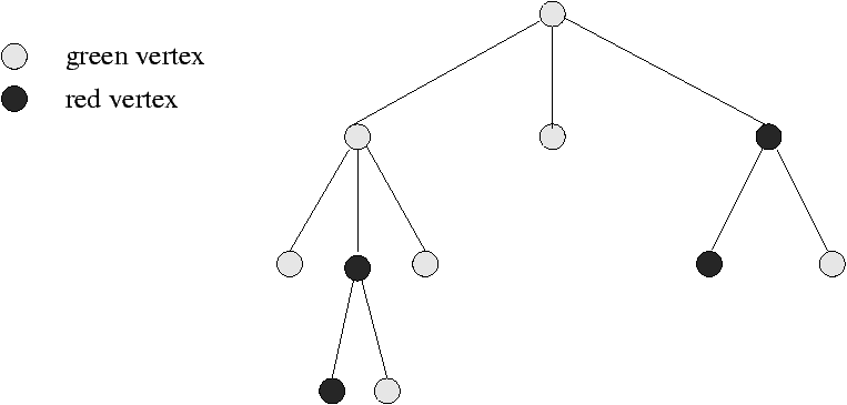
Consider a rooted plane tree where internal vertices can have two or three sons and are green or red, according to the following rules: (an example of such a tree is given below.)


Enumeration of such trees is best done by taking into account the colors of the vertices: let x1 and x2 mark the green and red vertices, and define w1(x1,x2) and w2 (x1,x2) as the functions enumerating the trees whose root is green (resp. red). These functions satisfy the system of equations
w1 (x1,x2) = x1 (1+ 3 w12 w2);     w2 (x1,x2) = x2 (1 + w1 w2).
Introducing the vectors x = (x1,x2) and w = (w1,w2) and the functions f1 (w) = 1 + 3 w12 w2 and f2 (w) = 1 + w1 w2, one obtains the system w1 (x) = x1 f1 (w); w2 (x) = x2 f2 (w). Such equations are very similar to those that can be solved in one dimension by Lagrange inversion, and it is natural to try and solve them with a suitable extension.

2   Multivariate Lagrange Inversion

In one dimension, Lagrange inversion is used for implicit equations of the type w(x) = x f(w(x)), with f(0)¹ 0: It relates the coefficients of a solution w(x), or of a function of w(x), as formal power series, to the coefficients of the simpler function f:
[ xn ] w(x) =
1
n
[ tn-1 ] f (t)n;      [ xn] g(w(x)) =
1
n
[ tn-1 ] g'(t) fn (t) .
Extensions to the multivariate case have been considered for some time; surveys can be found in the paper written some twelve years back by Gessel [6], or in the recent book by Bergeron, Labelle and Leroux [4]. The version presented below is due to Good [7]:
Theorem 1   Let x be a d-dimensional vector, g(x) and fi(x) (1 £ i £ d) be formal power series in x, s.t. fi (0) ¹ 0. Then the equations wi = xi fi (w) uniquely determine the wi as formal power series in x, and
[
t
n
 
] g(
w
(
t
)) = [
x
n
 
] æ
ç
ç
ç
è
g(
x
)
f
n
 
(
x
) ½
½
½
½
½
½
½
½
½
½
di,j -
xi fj(
x
)
fj (
x
) xi
½
½
½
½
½
½
½
½
½
½
ö
÷
÷
÷
ø
,
with di,j the Kronecker symbol, ||A|| the determinant of the matrix A, f = (f1,..., fd), and fn = f1n1··· fdnd.
The determinant in this formula leads to trouble when one tries to get asymptotic information from it. Let us consider the univariate case to see what the problem is.

For d=1, Good's formula applied to the equation w(x) = x f(w(x)) gives an identity equivalent to the one presented above:
[ xn ] w(x) = [ tn-1] æ
ç
ç
è
fn (t) æ
ç
ç
è
1-t
f'(t)
f(t)
ö
÷
÷
ø
ö
÷
÷
ø
.     (1)
When one wishes to obtain asymptotics, a natural tool is the saddle-point method, well suited to approximating coefficients of (variations on) large powers of functions; see for example [5] for a summary of results in this area. The idea is to use Cauchy's formula [ zn ] F(z) = ò F(z) z-n-1 dz, for F(z) = f(z)n (1-z f'(z) / f(z)), with an integration path that is a circle going through the saddle-point r0; r0 is itself is a perturbation of the saddle-point r1 that appears in the evaluation of the simpler coefficient [ xn ] fn (x). Now r1 is defined as the solution of the equation 1 - x f' (x) / f(x) =0, i.e. the integrand of the right part of (1) becomes zero close to r0!

With care, it should be possible to work this out for one variable, but the outlook for a multi-dimensional extension is not favorable, as we can expect cancellation of the determinant close to the integration paths. Instead, Bender and Richmond have proposed a new multivariate version, better suited to asymptotics; this formula will use the derivatives of a vector wrt a directed graph.

3   Differentiating a Vector wrt a Directed Graph

To define the partial of a vector relative to a directed graph, consider all trees with vertices 0, 1,..., d and edges directed to 0. There are (d+1)d-1 such trees; for example for d=2 there are three trees:


Now the derivative of a (d+1)-dimensional function f according to such a tree is a product on (d+1) terms, where fi is differentiated according to the incoming edges into the vertex labelled by i; this is best explained on the above example, with f = (f0,f1,f2):1

f
T1
=
2 f0
x1 x2
· f1 · f2;     
f
T2
=
f0
x2
· f1 ·
f2
x1
;     
f
T3
=
f0
x1
·
f2
x2
· f2.

4   The New Inversion Formula

Theorem 2   Under the assumptions of the former theorem,
[
t
n
 
] g (
w
(
t
)) = æ
ç
ç
è
d
Õ
i=1
ni ö
÷
÷
ø
-1


[
x
n
-
1
 
]
 
å
T
(g, f
n1
 
1
, ... , f
nd
 
d
)
T
,
where the sum is on the set of trees with d+1 vertices.

Proof. This result is proven in [3]; it relies on the simple formula n [ xn-1 ] f = [ xn ] f / x and on the expansion of a determinant. The terms are all positive as soon as the functions fi and g have positive coefficients; hence the coefficient [ tn ] g (w (t)), as a sum of (d+1)d-1 such terms, is itself positive and there are no more cancellations.


What do we obtain for the first values of d? For d=1, the only tree is 1 ® 0 and one gets back the classical formula. For d=2, g(t1,t2) is a function of two variables and
[ x
n1
 
1
x
n2
 
2
]
g(w1(x1,x2), w2(x1,x2)) =
1
n1 n2
[ t
n1-1
 
1
t
n2-1
 
2
]
 
å
T Î { T0, T1, T2 }
(g, f
n1
 
1
, f
n2
 
2
)
T
 
=
1
n1 n2
[ t
n1-1
 
1
t
n2-1
 
2
] æ
ç
ç
è
2 g
t1 t2
f
n1
 
1
f
n2
 
2
+
g
t2
f
n1
 
1
(f
n2
 
2
)
t1
+
g
t1
(f
n1
 
1
)
t2
f
n2
 
2
ö
÷
÷
ø
 
=
1
(n1-1) (n2-1)
[ t
n1
 
1
t
n2
 
2
] æ
ç
ç
è
f
n1
 
1
f
n2
 
2
h ö
÷
÷
ø
,
with (f1 and f2 are strictly positive at the saddle-points)
h:=
2 g
t1 t2
+ n2
g
t2
f2
t1
1
f2
+ n1
g
t1
f1
t2
1
f1
.

For general d, there is no determinant here, but a finite (although large!) sum of terms, each of which can be evaluated individually. The asymptotic value of [ tn ] g (w(x)) is obtained by adding the individual asymptotic values of the (d+1)d-1 terms.

It is possible to obtain a univariate local limit theorem for the number of red vertices in trees having a fixed number of vertices, or a bivariate local limit theorem for the joint distribution of the numbers of red and green vertices.

5   Local Limit Theorem

The usual approach towards a limiting theorem is through the covariance matrix (see for example a former paper by the same authors [1]); checking the non-degeneracy of this matrix leads to intricate conditions, which the authors try to bypass, by requiring instead the existence of a multivariate saddle-point. A local limit theorem holds whenever the functions g(x) and fi (x) (1£ i £ d) are analytic; there is also an existence condition on the exponents of the variables in the functions whose coefficients we are studying. Formally, this involves the lattice generated by the exponents k for which the coefficient of tk in fi is not zero; see [2] for a precise formulation.

For example, for the colored trees presented in Section 1, the only non-zero coefficients are obtained, besides k = (0,0), for k = (2,1) in f1, and for k = (1,1) in f2. The lattice generated by { (1,1), (2,1) } is N2; hence all the terms t1i1 t2i2 will appear in the function f1k1 f2k2.

The saddle-point condition is that we should be able to solve the system of d equations { ki = å1£ l £ d kl log fl / log gi} (with gi = esi).

We give the equations below for two variables, the better to understand what is going on, but it should be understood that it is more general and applies to d dimensions.

At some point, we have to compute a coefficient [ t1n1 t2n2 ] ( h f1n1 f2n2 ), where the functions h, f1 and f2 are on the variables t1 and t2. The way to do this is through a saddle-point approximation; more specifically we shall look at [ t1k1 t2k2 ] ( h f1n1 f2n2 ) for k1 and k2 of the same order as n1 and n2, but not necessarily equal. This coefficient can be written, by Cauchy's formula, as 1/(2ip)2 ò ò eh(t1,t2) dt1 dt2, with h = n1 log f1 + n2 log f2 - k1 log t1 - k2 log t2. Now the saddle-points are defined by the two equations h / t1 =0 and h / t2 =0, which give the two-dimensional system
k1 = n1 t1
f1
t1
1
f1
+ n2 t1
f2
t1
1
f2
;      k2 = n1 t2
f1
t2
1
f1
+ n2 t2
f2
t2
1
f2
.
Applied to our running example, this gives the system in t1 and t2
k1 = n1
6 t12 t2
1+3 t12 t2
+ n2
t1 t2
1+ t1 t2
;      k2 = n1
3 t12 t2
1+3 t12 t2
+ n2
t1 t2
1+ t1 t2
.
Define r:= k1 / k2; r Î]1,2[. Solving, we get
t1 =
(r -1)2
3 (2-r)
=: r1;      t2 =
3 (2-r)2
(r-1)3
=: r2.
This gives (k1,k2) = n (r / (1+r), 1/(1+r)). The covariance matrix is obtained by differentiation of log f, where f:= f1n1 f2n2, with f1 and f2 defined in Section 1. For example B1,1 is the value of t1 (log f) / t1 + t12 2 (log f) / t12, taken at the point (r1,r2), which gives B1,1 = n (r -1) (4+ 2 r - r2)/r (1+r). Similar computations give the other components of the covariance matrix:
n
r -1
r (1+r)
é
ë
4+2r - r2 2+2r - r2
2+2r-r2 1+2r-r2
ù
û
.

References

[1]
Bender (Edward A.) and Richmond (L. Bruce). -- Central and local limit theorems applied to asymptotic enumeration. II. Multivariate generating functions. Journal of Combinatorial Theory. Series A, vol. 34, n°3, 1983, pp. 255--265.

[2]
Bender (Edward A.) and Richmond (L. Bruce). -- Multivariate asymptotics for products of large powers with applications to Lagrange inversion. -- Technical Report n°Technical Report 98-10, Faculty of Mathematics, University of Waterloo, 1998.

[3]
Bender (Edward A.) and Richmond (L. Bruce). -- A multivariate Lagrange inversion formula for asymptotic calculations. Electronic Journal of Combinatorics, vol. 5, n°1, 1998, pp. Research Paper 33, 4 pp. (electronic).

[4]
Bergeron (F.), Labelle (G.), and Leroux (P.). -- Combinatorial species and tree-like structures. -- Cambridge University Press, Cambridge, 1998, Encyclopedia of Mathematics and its Applications, vol. 67, xx+457p. Translated from the 1994 French original by Margaret Readdy, With a foreword by Gian-Carlo Rota.

[5]
Gardy (Danièle). -- Some results on the asymptotic behaviour of coefficients of large powers of functions. Discrete Mathematics, vol. 139, n°1-3, 1995, pp. 189--217.

[6]
Gessel (Ira M.). -- A combinatorial proof of the multivariable Lagrange inversion formula. Journal of Combinatorial Theory. Series A, vol. 45, n°2, 1987, pp. 178--195.

[7]
Good (I. J.). -- The generalization of Lagrange's expansion and the enumeration of trees. Proceedings of the Cambridge Philosical Society, vol. 61, 1965, pp. 499--517.

[8]
Hwang (Hsien-Kuei). -- On convergence rates in the central limit theorems for combinatorial structures. European Journal of Combinatorics, vol. 19, n°3, 1998, pp. 329--343.

1
Although the definition is more general, trees are the only graphs considered here.

This document was translated from LATEX by HEVEA.