Solvability of Some Combinatorial Problems

Solvability of Some Combinatorial Problems

Anthony Guttmann

Department of Mathematics, University of Melbourne, Australia

Algorithms Seminar

December 2, 1996

[summary by Dominique Gouyou-Beauchamps]

A properly typeset version of this document is available in postscript and in pdf.

If some fonts do not look right on your screen, this might be fixed by configuring your browser (see the documentation here).

Abstract

Some of the most famous results in mathematics involve a proof of the intrinsic unsolvability of certain problems---such as the roots of a general quintic. In mathematical physics such results are largely unknown. I will describe a powerful numerical technique that provides compelling evidence for (but is not a proof of) the unsolvability of a wide variety of classical, unsolved problems in Statistical Mechanics and Combinatorics, in terms of the ``standard'' functions of mathematical physics (including D-finite functions).

1 Inversion relation

An inversion relation is a functional relation satisfied by a transfer matrix, and hence satisfied by the partition function (and hence satisfied by correlation functions). It is connected with concepts of integrability and the star-triangle relation (Onsager [7], Baxter [1], Maillard, Stroganoff [8]). An inversion relation exists for many unsolved models e.g., 2d Ising model in a magnetic field, 2d Potts model (non-critical), 3d Ising model (H=0) etc. It gives a strong constraint on the partition function and correlation function.

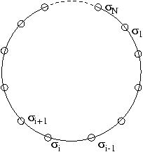
We first consider the transfer matrix for the Ising model with d=1 and H¹ 0 (see [4, 3]). The free energy is

-b H =K

å

<i,j>
s_is_j+H

å

i
s_i
with j=i+1, s_i=± 1 and s_N+1=s₁. The interaction energy between each pair of successive atoms depends on whether their internal coordinates are alike or different: u(1,1)=u(-1,-1)=-u(1,-1)=-u(-1,1)=-K. The canonical partition function Z(K,H) of the model is defined as

Z(K,H)

-b H

s₁,s₂,...,s_N=± 1

exp

æ
ç
ç
è

u(s_k, s_k+1)-Hs_k

ö
÷
÷
ø

s₁,s₂,... ,s_N=± 1

exp

æ
ç
ç
è

(Ks_k s_k+1+Hs_k)

ö
÷
÷
ø

We express this sum in terms of a transfer matrix T^~ whose elements are

(s |

|s ')=e

-u(s ,s ') +Hd

s ,s '

= e

Ks s '+Hd

s ,s '

where d is the Kronecker delta function. Then the summation over (s₁,s₂,... ,s_N) is equivalent to matrix multiplication, and we obtain

Z(K,H)=

s₁

(s₁|

^N|s₁)= Tr

(

^N).

The transfer matrix T^~ is

æ
è

e^K+H	e^-K
e^-K	e^K+H

ö
ø

and by inspection

(K,H)

(K+

,-H)=2isinh

(2K)

and the partition function verifies

Z(K,H)Z(K+

,-H)=2isinh (2K).

This inversion relation can be confirmed taking the partition function definition:

Z(K,H)=e^Kcosh H+(e^2Ksinh ²H+e^-2K)^1/2.

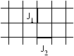
For the anisotropic 2d Ising model [7], the free energy is

-b H =K₁

å

<i,j>
⁽¹⁾s_is_j +K₂

å

<i,j>
⁽²⁾s_is_j.
The diagonal-to-diagonal transfer matrix leads to the following inversion relation for the partition function

Z(K₁,K₂)Z(-K₁,K₂+

ip

2
)=2isinh (2K₂).

Let t₁=tanh (J₁/kT), t₂=tanh (J₂/kT). We define the reduced partition function

L (t₁,t₂)=(2cosh K₁cosh K₂)^-1Z(K₁,K₂).

This satisfies the functional relation

ln L (t₁,t₂)+ln L (1/t₁,-t₂)=ln (1-t₂²).

Now a series expansions gives:

ln L (t₁,t₂)

m,n

a_mnt₁^2mt₂²ⁿ

=t₁²t₂²+ t₁⁴t₂²+t₁²t₂⁴+t₁⁶t₂²+t₁²t₂⁶+

t₁⁴t₂⁴ +t₁⁸t₂²+t₁²t₂⁸+5t₁⁶t₂⁴+5t₁⁴t₂⁶+···

and a partial sum over m yields:

L (t₁,t₂)=

n=1

R_n(t₁²)t₂²ⁿ

where R_n(t₁²)=å_ma_m,nt₁^2m is the generating functions for graphs with 2n vertical steps. From graphical expansion, we obtain

R₁(t₁²)=

t₁²

1-t₁²

, R₂(t₁²)=

t₁²-1/2t₁⁴+1/2t₁⁶

(1-t₁²)³

and from higher order terms we see a pattern [1]

R_n(t₁²)=

P_2n-1(t₁²)

(1-t₁²)^2n-1

The fact that the only singularity of the denominator occurs at t₁²=1, plus inversion relation, plus obvious symmetry (L (t₁,t₂)=L (t₂,t₁)) completely determines the polynomials P_2n-1(t²), and hence implicitly yields the Onsager solution [1].

The zero-field susceptibility of the triangular lattice Ising model [5], with coupling constants K₁, K₂, K₃, and t_i=tanh (K_i), satisfies an inversion relation [6] c (t₁,t₂,t₃)+c (-t₁,-t₂,1/t₃)=0. Since the anisotropic square lattice can be obtained by setting one of the anisotropic coupling constants to zero, it follows that the anisotropic square lattice susceptibility satisfies the inversion relation c (t₁,t₂)+c (1/t₁,-t₂)=0, as well as the symmetry relation c (t₁,t₂)=c (t₂,t₁)=0. Writing the high temperature expansion

c (t₁,t₂)=

m,n=0

c_mnt₁^mt₂ⁿ=

n=0

H_n(t₁)t₂ⁿ,

the inversion relation then implies H_n(t₁)+(-1)ⁿH_n(1/t₁)=0. The first five values of H_n(x) were given in [5], and I. G. Enting and A. J. Guttmann recently reported the calculation of H_n(x) for n£ 14.

H₀(t)=

1+t

1-t

, H₁(t)=

2(1+t)²

(1-t)²

H₂(t)=

2(1+6t+8t²+6t³+t⁴)

(1-t)³(1+t)

, H₃(t)=

2(1+8t+10t²+8t³+t⁴)

(1-t)⁴

H₄(t)=

2(1+t¹⁰+15(t+t⁹)+71(t²+t⁸)+192(t³+t⁷)+326(t⁴+t⁶)+388t⁵)

(1-t³)(1-t)⁴(1+t)³

,...,

H₁₀(t)=

2(1+t³⁴+45(t+t³³)+758(t²+t³²)+... + 1075878111(t¹⁶+t¹⁸)+1131919146t¹⁷)

(1-t³)⁷(1-t)⁴(1+t)⁹

In all cases enumerated, the numerator polynomial is unimodal and symmetric with positive coefficients. The numerator and denominator polynomials (with no common factors) are of equal degree. The susceptibility of the Ising model can be expressed as an expansion in terms of (2k+1) particle excitations [9]. Hence the structure of the denominator is clear. The contribution of the terms from the 2k+1 particle excitations, which first contribute at, say, O(t^2m), correspond to poles at t^2k+1=1 in H_m(t) in the anisotropic expansion above. We can identify the first occurrence of the term (1-t^2k+1) in the denominator with the first occurrence of a (2k+1) particle excitation. From this observation, we see that structure of H_n(t) is that of a rational function whose poles all lie on the unit circle in the complex t plane, so that poles become dense on the unit circle as n gets large.

Hence c (t₁,t₂) as a function of t₁ for t₂ fixed (i.) has a natural boundary; (ii.) is not algebraic; and (iii). cannot be expressed in terms of the ``usual'' functions of mathematical physics, such as elliptic integrals, hypergeometric functions etc.

One family of solutions that does suggest itself as a possible candidate is the family of q-deformations of standard functions. Several examples are known already in the work done in both Camberra and Melbourne, as well as Bordeaux and various other places.

Now this suggests a powerful tool: generalize to the anisotropic model and study the distribution of zeros in the denominator of the analogue of H_n functions. Then we can distinguish between those that appear to be solvable in terms of standard functions---when there is just a finite number of singularities on the unit circle---and those which are not, with an infinite number of such singularities.

2 The anisotropic model

We have applied this approach to a number of other unsolved problems in statistical mechanics of two dimensional systems.

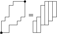
Staircase polygons (or parallelogram polyominoes)

H_m(x²) is the generating function for staircase polygons with 2m vertical bonds.

H₁(x²)

=

x²

1-x²
,
H₂(x²)

=

x²

(1-x²)³
,

H₃(x²)

=

x²(1+x²)

(1-x²)⁵
,
H₄(x²)

=

x²(1+3x²+x⁴)

(1-x²)⁷
,

H₅(x²)=

x²(1+6x²+6x⁴+x⁶)

(1-x²)⁹

,..., H_m(x²)=

x²S_m(x²)

(1-x²)^2m-1

S_m(x²) is a symmetric unimodal polynomial of degree (m-2). H_m(x²) satisfies the inversion relation

H_m(x²)+x^-2(m-1)H_m(1/x²)=0

and it follows that the generating function P(x,y) verifies

P(x,y)=

x²y²

1-x²

+G(x,y) where G(x,y)=-x²G(1/x,y/x) and P(x,y)=P(y,x) .

The complete solution is implicitly determined by these relations, initial conditions and the fact that the only singularity of the denominator occurs at x²=1.

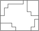
Convex polygons

H_n(x²) is the generating function for convex polygons with 2n vertical bonds.

H₁(x²)=

x²

1-x²
, H₂(x²)=

x²(1+x²)²

(1-x²)³
,

H₃(x²)=

x²(1+8x²+13x⁴+2x⁶)

(1-x²)⁵
,

H_n(x²)=

x²T_n(x²)

(1-x²)^2n-1
.

T_n is a unimodal (with positive coefficients), asymmetric (n>2) polynomial of degree n. Absence of symmetry precludes solution by this method.

Row convex polygons

P(x,y)¹ P(y,x),

P(x,y)=

å

n
x²ⁿH_n(y²)=

å

m
y^2mA(x²).

H_n(y²)=T_n(y²)/(1-y²)^2n-1 where T_n(y²) is a symmetric, unimodal polynomial of degree 2n-1 in y² and H_n(y²)=-H_n(1/y²) so P(x,y)+P(x,1/y)=0.

A_m(x²)=U_m(x²)/(1-x²)^2m-1 where U_m(x²) is an asymmetric (m>2), unimodal polynomial of degree 2n-1 in x². Absence of symmetry precludes solution by this method.

3 choice polygons

The number of 3 choice polygons of 2n steps grows like

2^2n-5

(np)^1/2

(15.13161+

3(3)^1/2

ln n).

If H_n(y²) is the generating function for 3 choice polygons with 2n horizontal bonds, then the general generating function P(x,y) for 3 choice polygons satisfies

P(x,y)=

å

n
x²ⁿH_n(y²).

H₂(y²)=

1

(1-y²)³
,

H₃(y²)=

3+2y²

(1-y²)⁵
,

H₄(y²)=

6+19y²+15y⁴+4y⁶)

(1-y²)⁷(1+y²)
,

H₅(y²)=

10+75y²+194y⁴+237y⁶+161y⁸+66y¹⁰-5y¹²-12y¹⁴+16y¹⁶ -6y²⁰+2y²²

(1-y²)⁹(1+y²)³

The denominator in general is

H_n=(1-y²)^2n-1(1+y²)^2n-7=(1-y²)⁶(1-y⁴)^2n-7 for n>3.

This is consistent with solvability and the solution is probably D-finite.

Square lattice polygons (I. Enting)

We have no inversion relation for this model but P(x,y)=P(y,x). We define R_n(x²) by the relation

P(x,y)=

n=1

R_n(x²)y²ⁿ.

Numerators of the R_n(x²) are unimodal, positive, but not symmetric. The degree of the numerator is equal to that of the denominator. The denominator is (1-x²)^2n-1 for n£ 4, but for n>4 powers of 1-x⁴ enter, and for n>6 we see powers of 1-x⁶ entering, while n=8 marks the first occurrence of powers of 1-x⁸ [3].

Self avoiding walks on square lattice (A. Conway)

We have no inversion relation for this model. We define H_n(x) by the relation

C(x,y)=

n=0

H_n(x)yⁿ.

H_n(x) (now known up to n=12) is equal to A_n^m/B_n^m where A_n^m and B_n^m are polynomials of degree m, A_n^m is unimodal and B_n^m is equal to

B_n^m(x)=(1-x)

(1+x)

(1+x+x²)

(1+x²)

Up to n=9, we have a=n+1, b=2(ë n/2û) with n>1, g =n-4 with n>4 and d=1,1,3 for 9³ n>6 [2].

Honeycomb polygons (brickwork)

H_n(x²)=P_n(x²)/Q_n(x²). The denominator pattern is quite regular. The denominators always have zeros only on the unit circle [3], just at x²=1 for n£ 3, with powers of 1-x⁴ appearing at n=4, powers of 1-x⁶ entering at n=7 and so on. Numerators are positive coefficients, unimodal, but not symmetric. The numerator and denominator are not of equal degree.

Anisotropic, hexagonal directed animals (A. J. Guttmann and A. R. Conway)

The generating function is G(z)=å_{n³ 1}a_nzⁿ where a_n is the number of animals with n sites and one source. For square and triangular lattice Dhar showed

that the generating function is algebraic;
that the model is equivalent to hard squares in some sense;
a_n~µ ⁿ/(n)^1/2 with µ =3 for the square lattice and µ =4 for the triangular lattice.

For the hexagonal lattice, Dhar found µ =2.0252± 0.0005 and no generating function could be found. We extended the series to 99 terms, found µ =2.025131± 0.000005 but no exact solution. The study of an isotropic model G(x,y)=å_{n³ 0}H_n(x)yⁿ gives H_n(x)=N_n(x)/D_n(x) where the denominator pattern can be guessed. In this case, we have the symmetry G(x,y)=G(y,x).

References

[1]: Baxter (R. J.). -- Exactly solved models. In Cohen (E. G. D.) (editor), Fundamental Problems in Statistical Mechanics. vol. 5. -- Amsterdam, 1980. Proceedings of the 1980 Enschede Summer School.
[2]: Conway (A. R.) and Guttmann (A. J.). -- Square lattice self-avoiding walks and corrections to scaling. Physical Review Letters, vol. 77, n°26, 1996, pp. 5284--5287.
[3]: Guttmann (A. J.) and Enting (I. G.). -- Inversion relations, the Ising model and self-avoiding polygons. Nuclear Physics (Proc. Suppl.), vol. 47, 1996, pp. 735--738.
[4]: Guttmann (A. J.) and Enting (I. G.). -- Solvability of some statistical mechanical systems. Physical Review Letters, vol. 76, n°3, 1996, pp. 344--347.
[5]: Hansel (D.), Maillard (J. M.), Oitmaa (J.), and Velga (M. J.). -- Analytical properties of the anisotropic cubic Ising model. Journal of Statistical Physics, vol. 48, n°1/2, 1987, pp. 69--80.
[6]: Jaekel (M. T.) and Maillard (J. M.). -- A disorder solution for a cubic Ising model. Journal of Physics Series A, vol. 18, 1985, pp. 641--651.
[7]: Onsager (L.). -- Crystal statistics. I. A two dimensional model with an order-disorder transition. Physical Review, vol. 65, 1944, p. 117.
[8]: Stroganov (Y. G.). -- A new calculation method for partition functions in some lattice models. Physical Letters, vol. 74A, n°1,2, 1979, pp. 116--118.
[9]: Wu (T. T.), McCoy (B. M.), Tracy (C. A.), and Barouch (E.). -- Spin-spin correlation functions for the two-dimensional Ising model: Exact theory in the scaling region. Physical Review B, vol. 13, 1976, pp. 316--374.

This document was translated from L^AT_EX by H^EV^EA.