ENUMERATION OF PLANAR CONFIGURATIONS
IN COMPUTATIONAL GEOMETRY
Philippe Flajolet
(Version of January 15, 1997)
Consider
![]() points on a circle that define a convex polygon. The enumeration of geometric configurations that can be superimposed on these points has a dignified history. In 1753, Euler solved the problem of counting the number of possible triangulations of a convex
points on a circle that define a convex polygon. The enumeration of geometric configurations that can be superimposed on these points has a dignified history. In 1753, Euler solved the problem of counting the number of possible triangulations of a convex
![]() -gon while inventing the concept of generating function for this particular combinatorial enumeration problem. Since then, many configurations have been enumerated; see Comtet's
Advanced Combinatorics,
p. 74 for a discussion of works of Prouhet 1886, Jordan 1920, Guy 1967.
-gon while inventing the concept of generating function for this particular combinatorial enumeration problem. Since then, many configurations have been enumerated; see Comtet's
Advanced Combinatorics,
p. 74 for a discussion of works of Prouhet 1886, Jordan 1920, Guy 1967.
Till recently, any new enumerative result was basically a research paper, and some of the applications discussed below have required several pages of recurrence manipulations. In this report, we take inspiration from a recent memo of Noy (September 1996) and show that many such results can be derived automatically using the Maple system and the packages Combstruct and Gfun . This worsheet is meant as a simple introduction to Combstruct specifications as well as to basic experimental computations that may accompany them.
Euler's counting of triangulations
Problem
Find the number of ways of cutting up a convex
![]() -gon into n triangles by means of
-gon into n triangles by means of
![]() non-intersecting diagonals.
non-intersecting diagonals.
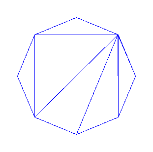
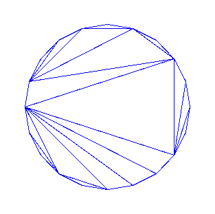
Here are examples of triangulations of the octogon and of the icosagon.


Specification
A triangulation decomposes into three components:
- the "root" triangle uniquely defined uniquely by the fact that it contains the edge with smallest numbers (
![]() initially);
initially);
- the left and right subtriangulations defined by their position with respect to the root triangle.
First, we load the combstruct package:
> with(combstruct);
![]()
![]()
In writing a specification, we take the atomic symbol
![]() to denote a traingle,
to denote a traingle,
![]() being an arbitrary triangulation. One must be careful to isolate one-sided triangulations, where either the left or the right subtriangulations may be empty. Thus, the grammar is
being an arbitrary triangulation. One must be careful to isolate one-sided triangulations, where either the left or the right subtriangulations may be empty. Thus, the grammar is
> triang:=[T,{T=Union(Z,Prod(Epsilon,Z,T),Prod(T,Z,Epsilon),Prod(T,Z,T))},unlabelled]:
This specification is clearly reminiscent of binary search trees.
Counting.
Now, we can count the number of triangulations of size 100:
> count(triang,size=100);
Here the system takes a couple of seconds to set up (once and for all!) complete counting tables till size equal to 100.
![]()
![]()
In particular, the first few values are
> seq(count(triang,size=i),i=0..20);
![]()
![]()
![]()
These numbers are known as the Catalan numbers in the honor of the French and Belgian mathematician who worked out their main properties in the 1850's.
Random generation.
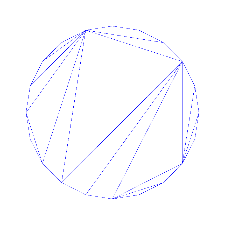
We can draw a triangulation at random amongst those of any given size. Note that uniformity is granted a priori by the algorithms contained in the combstruct package. Naturally, the output is in the format dictated by the specification. Here is a triangulation of size 10, that is to say, comprised of 10 triangles, and corresponding to a dodecagon.
> draw(triang,size=10);
![]()
![]()
Since the objects generated are standard Maple objects, we can manipulate them and in particular construct plots to visualise them. Here is a set of procedures to construct the list of edges of a triangulation.
> size:=proc(t) convert(map(size,t),`+`) end: size(Epsilon):=0: size(Z):=1:
>
set_edges:=proc(tree,org,edge_set) local se1,se2;
if tree=Epsilon then
org,org,edge_set union {[org,org+1]}
elif tree=Z then
org,org+1,edge_set union {[org,org+1],[org+1,org+2],[org+2,org]}
else
se1:=set_edges(op(1,tree),org,edge_set);
se2:=set_edges(op(3,tree),se1[2]+1,se1[3]);
se1[1],se2[2],se2[3] union {[se1[1],se2[2]+1]}
fi
end:
> plott:=proc(n) plot([op(map2(map,[cos,sin],expand(map(`*`,set_edges(draw(triang,size=n-2),0,{})[3],2*Pi/n))))],color=blue,axes=NONE) end:
> plott(20);

Exhaustive generation.
With the December 1996 release of Combstruct , we may also list exhautively all configurations of a given size. This proves useful for exhaustive testing of small cases, though there are physical limitations owing to the exponential growth of the number of cases.
> tr4:=allstructs(triang,size=4);
![]()
![]()
![]()
![]()
![]()
![]()
![]()
![]()
![]()
![]()
![]()
We found 14 objects, as we should.
Generating function equations.
Again, this uses the December 1996 release of Combstruct. We may form the generating function equations associated to a given specification, as follows:
> gfeqns(op(2,triang),unlabelled,z);
![]()
> gfsys:=gfsolve(op(2,triang),unlabelled,z);
![[Maple Math]](nc-configs32.gif)
Here, the solution could be obtained explicitly. Correctness can be checked by a Taylor expansion, comparing with what combstruct[count] gives us.
> op([1,2],"); series(",z=0,12);
![[Maple Math]](nc-configs33.gif)
![]()
![]()
> seq(count(triang,size=n),n=0..10);
![]()
Alternatively, an arbitrary system of generating function equations can be solved by means of combstruct[gfseries] , even when no closed form is available.
> gfseries(op(2..3,triang),z,[[z]],6);
![]()
![]()
![]()
![]()
Noy's counting of non-crossing trees
Problem.
Find the number of trees (called non-crossing trees) that can be built on the n vertices on the
![]() -gon, assuming that no edges of the tree intersect.
-gon, assuming that no edges of the tree intersect.
Specification.
View node number 0 as the root, the vertices being number from 0 to
![]() . An arbitrary number of edges connect the root to other nodes. At each such node
. An arbitrary number of edges connect the root to other nodes. At each such node
![]() connected to the root, there is a "butterfly", defined by two noncrossing trees attached to
connected to the root, there is a "butterfly", defined by two noncrossing trees attached to
![]() (one non-crossing tree to the left of the edges
(one non-crossing tree to the left of the edges
![]() , the other to the right). We let
, the other to the right). We let
![]() denote non-crossing (NC) trees,
denote non-crossing (NC) trees,
![]() denote forests defined by pruning the root of a
denote forests defined by pruning the root of a
![]() -tree, and
-tree, and
![]() denote a butterfly. The specification results.
denote a butterfly. The specification results.
> nctree:=[T,{T=Prod(Z,F),F=Sequence(B),B=Prod(F,Z,F)},unlabelled]:
> seq(count(nctree,size=i),i=0..20);
![]()
![]()
![]()
Random generation, exhaustive generation.
We draw objects at random with combstruct[draw] . Here is a random NC-tree.
> draw(nctree,size=8);
![]()
![]()
![]()
![]()
Guessing counts with Maple.
At this stage, we ask ourselves whether a closed form expression may exist. First, let us examine the way we might proceed in a simple case, using Maple. Consider for instance the number of NC-trees of size 30 and try to factor it.
> ifactor(count(nctree,size=30));
![]()
![]()
We observe that the count is a highly composite number that involves all the prime numbers between 31 and 83. This is a strong indication that a closed form involving factorials or binomial coefficients should exist. The pattern can then be guessed by taking successive quotients.
> seq([n,ifactor(count(nctree,size=n+1)/count(nctree,size=n))],n=1..15);
![[Maple Math]](nc-configs59.gif)
![[Maple Math]](nc-configs60.gif)
![[Maple Math]](nc-configs61.gif)
![[Maple Math]](nc-configs62.gif)
![[Maple Math]](nc-configs63.gif)
The ratios clearly involve
![]() and
and
![]() in the denominator, at least whenever these are primes. We thus try:
in the denominator, at least whenever these are primes. We thus try:
> seq([n,ifactor(n*(2*n+1)*count(nctree,size=n+1)/count(nctree,size=n))],n=1..15);
![]()
![]()
![]()
![]()
![]()
![]()
![]()
The numerators now seem to involve
![]() and
and
![]() . Thus we try next
. Thus we try next
> seq([n,ifactor(n*(2*n+1)/(3*n-1)/(3*n-2)*count(nctree,size=n+1)/count(nctree,size=n))],n=1..15);
![[Maple Math]](nc-configs75.gif)
![[Maple Math]](nc-configs76.gif)
![[Maple Math]](nc-configs77.gif)
We have thus found empirically evidence for the conjecture that the counts satisfy
> u(n+1)=3/2*n*(2*n+1)/(3*n-1)/(3*n-2)*u(n);
![[Maple Math]](nc-configs78.gif)
This can be solved by means of the Maple command rsolve , suggesting a closed binomial form for the coefficients.
> rsolve({",u(1)=1},u);
![[Maple Math]](nc-configs79.gif)
Naturally, we succeeded here only because the counts admit a direct product form.
Guessing counts with Gfun.
Our guessing task is greatly simplified if we appeal to the Gfun package that determines automatically recurrences for sequences and differential equations for the corresponding generating functions that match a given set of initial data.
> with(gfun);
![]()
![]()
![]()
![]()
![]()
![]()
![]()
![]()
![]()
![]()
![]()
![]()
![]()
First, we build a list of small values:
> l:=[seq(count(nctree,size=n),n=0..20)];
![]()
![]()
![]()
![]()
The procedure gfun[listtorec] finds automatically a plausible recurrence with polynomial coefficients, provided such a form exists; similarly, the procedure gfun[listtodiffeq] finds automatically a plausible differential equation with polynomial coefficients, provided such a form exists.
> listtorec(l,u(n));
![]()
![]()
> listtodiffeq(l,U(z));
![[Maple Math]](nc-configs99.gif)
![[Maple Math]](nc-configs100.gif)
This candidate equation can be passed for possible solution to Maple's dsolve.
> dsolve(op(1,"),U(z));
![[Maple Math]](nc-configs101.gif)
Proving solutions with Combstruct.
With the version of December 1996, we can find automatically a system of equations and in this particular case, an explicit solution.
> gfeqns(op(2..3,nctree),z);
![[Maple Math]](nc-configs102.gif)
![[Maple Math]](nc-configs103.gif)
> nctree_sys:=gfsolve(op(2..3,nctree),z);
![]()
![]()
![]()
This tells us in particular that the generating function of non-crossing trees is
> nctree_gf:=subs(nctree_sys,B(z));
![]()
> series(nctree_gf,z=0,12);
![]()
![]()
Conclusion .
In particular, we have obtained automatically one of the theorems of Noy (1994):
Theorem . The generating function of non crossing trees satisfies the equation
![[Maple Math]](nc-configs110.gif) .
.
The number of trees with
![]() nodes is
nodes is
![[Maple Math]](nc-configs112.gif) .
.
The result of combstruct[gfsolve] gives a valid proof of the generating function equation. The result of gfun[guessgf] followed by gfun[listtodiffeq] is a priori only heuristic. However, once a candidate recurrence or differential equation has been found, it may then rigorously be checked from withing gfun itself.
First, we compute automatically a differential equation from the generating function.
> algfuntoalgeq(nctree_gf,Y(z));
![]()
> algeqtodiffeq(",Y(z));
![[Maple Math]](nc-configs114.gif)
![[Maple Math]](nc-configs115.gif)
This result has proven value and it coincides with the differential equation that was previously "guessed". Thus, the theorem has been established "automatically"...
Comtet's counting of slicings.
Problem.
Given
![]() points on a circle, count the number of slicings, that is to say, graphs cons
isting of
points on a circle, count the number of slicings, that is to say, graphs cons
isting of
![[Maple Math]](nc-configs117.gif) edges that do not intersect inside the circle.
edges that do not intersect inside the circle.
Specification, random generation, and counting.
Consider first the case of an even number of vertices. A slicing decomposes into a central edge (initially, the edge that contains vertex 0) and into a left and right slicing that are each of a similar nature. This is readily specified as follows.
> sl0:={Edge=Prod(Z,Z),S=Union(Epsilon,Prod(S,Edge,S))}: slicing:=[S,sl0,unlabelled]:
> seq(count(slicing,size=n),n=0..20);
![]()
![]()
Our old friends, the Catalan numbers strike again.
An interest of the method is to allow for the counting of odd slicings, where one has a free unattached point. The following specification just says that the "free point" lies somewhere either left or right or at the root of the slicing.
> sl1:=sl0 union {Free=Z, S1=Union(Prod(S1,Edge,S),Prod(S,Edge,S1),Prod(S,Free,S))}: slicing1:=[S1,sl1,unlabelled]:
> seq(count(slicing1,size=n),n=0..20);
![]()
![]()
> draw(slicing1,size=20);
Error, (in combstruct/drawgrammar) there is no structure of this size
There, the system has recognized the absence of any structure of even size. Everything goes well with an odd size.
> draw(slicing1,size=19);
![]()
![]()
![]()
![]()
Jordan's couting of non-crossing Hamiltonian paths.
Problem.
Given
![]() points on a circle, determine the number of hamiltonian paths that have no crossing edges
.
points on a circle, determine the number of hamiltonian paths that have no crossing edges
.
Specification, random generation and couting.
We discuss here the simpler problem of specifying non-crossing hamiltonian paths that start at the designated root node of index 0. An initial segment of such a path can be continued in two ways, either by moving to the "next" point (an
![]() -move) away from the root, or by crossing over to the opposite side (an
-move) away from the root, or by crossing over to the opposite side (an
![]() -move). The final step (the
-move). The final step (the
![]() -step) is fully determined by the context. Thus, the specification is:
-step) is fully determined by the context. Thus, the specification is:
> ham_path:=[H,{H=Prod(Sequence(Union(N,X)),F),F=Z,N=Z,X=Z},unlabelled]:
We count, draw, etc. For instance:
> seq(count(ham_path,size=n),n=0..20);
![]()
![]()
Naturally, the result is the powers of two. We leave it as an exercise to prove that the number of unconstrained hamiltonian paths is
![[Maple Math]](nc-configs132.gif) . The idea is to decompose such paths as either starting right, or left, or as a gluing (with suitable constraints) of two paths that emenate from the root node.
. The idea is to decompose such paths as either starting right, or left, or as a gluing (with suitable constraints) of two paths that emenate from the root node.
Other non-crossing configurations.
Discussion.
By the same principles, it is possible to enumerate, list exhautively, draw at random, etc, a large number of geometrical configurations. Examples are general non-crossing graphs, forests, dissections, trees and graphs of bounded degree (Noy , September1996). We discuss here the case of forest.
Problem.
How many forests of trees with no crossing edges can be built from
![]() points on a circle?
points on a circle?
Specification, counting and generating functions.
A forest has a skeletton that is defined as the non-crossing tree that contains the vertex of smallest index. A (possibly empty) forest is then attached to each node of the skeleton. Thus forests are recursively definable as non-crossing trees of forests.
The corresponding specification is thus derived from that of NC-trees.
> forest:=[F,{F=Union(Epsilon,T),T=Prod(Z1,P),P=Sequence(B),B=Prod(P,Z1,P),Z1=Prod(Z,F)},unlabelled]:
> seq(count(forest,size=n),n=0..20);
![]()
![]()
![]()
![]()
> draw(forest,size=20);
![]()
![]()
![]()
![]()
![]()
![]()
![]()
![]()
![]()
![]()
![]()
> forest_sys:=gfsolve(op(2..3,forest),z);
![[Maple Math]](nc-configs149.gif)
![[Maple Math]](nc-configs150.gif)
![[Maple Math]](nc-configs151.gif)
![[Maple Math]](nc-configs152.gif)
![]()
![[Maple Math]](nc-configs154.gif)
> evala(subs(forest_sys,F(z)));
![]()
![]()
![]()
We automatically obtain a theorem of Noy (1996).
> series(",z);
![]()
Conclusions.
We have demonstrated the way Combstruct can be used to do experimental combinatorics. In conjunction with Gfun , it can help generate conjectures and even derive automatic proofs of theorems in combinatorics.