Combinatorics of Non-Crossing Configurations

F. Cazals, August 1997

Generalities

Non-Crossing configurations

Take points equally spaced on the unit circle, and draw chords between these points with the constraint that no two chords cross one-another. The resulting configuration is called a non-crossing configuration and the study of such entities originates in the work of Euler and Segner in 1753 for counting triangulations of a n-gon. Since then several types of such configurations have been defined, and for example the presence/absence of cycles and the number of connected components in a given configuration define the classes of trees and forests, connected graphs and general graphs. In addition to be of combinatorial interest per se, these configurations are also important for algorithmic problems arising in computer graphics or computational geometry where they provide simple models for real-world situations.

If historically the study of these configurations has been carried out one at a time, it turns out that they all fit in the model of algebraic and analytic combinatorics and are thus amenable to a unified treatment. More precisely, they can be defined in terms of grammars, from which the generating functions can automatically be obtained and used to asymptotically analyse the number of configurations, the number of connected components, etc.

The goal of this worksheet is to present this chain, from the grammars specification using combstruct, to the asymptotics of algebraic functions using some features of gfun, together with some plots of random configurations and of the singularities determining the asymptotic behaviour. The reader is referred to [FlaNo97] for the details.

The worksheet is organized as follows. In the rest of this section we define a few functions of null combinatorial interest but that we shall need to plot random configurations. In section two we present the grammar specifications for 6 of the main non-crossing configurations together with some plots of random configurations. And section three is devoted to the asymptotic machinery used to count the number of configurations of a given size, as well as a comparison between the asymptotic estimates and the exact values.

But to begin with, we first load the combstruct, gfun and plots libraries:

> with(combstruct):with(gfun):with(plots):

Appendix

Again, we define here a few functions we shall need to plot NC configurations. The first one returns the number of atoms in a structure, that is its size:

> size:=proc(t) convert(map(size, t), `+`) end:size(Epsilon):=0: size(Z):=1:

Since a configuration is defined by edges drawn between points equally spaced on the unit circle, we first show how to retrieve these pairs of indices from the grammars to be defined in the next section:

Collecting the edges of a NC-tree

Since a tree T satisfies T=Product (Z, Sequence(Butterflies)), to plot it we just have to collect its edges which are pairs of indices in 0..n-1:

> plotTree:= proc(aTree) local r, nbVertices;
#--op returns the Sequence; 0 is the index of the root on the circle;
#--1 indicates that the butterflies attached to the root are counted as a
#--right wing
r:=getTreeEdges(op(2, aTree), 0, 1);
nbVertices:=size(aTree);

plotSetOfEdges(r, nbVertices)
end:

The parameters of getTreeEdges are the following: aSeqOfBtf is a sequence of butterflies; rootIdx is the index of the vertex this sequence is attached to; leftRight (-1 or +1) indicates if this sequence is a left/right wing of the bug. The algorithm works as follows:

1.We first compute the indices of the apex vertices of the butterflies

2.For a given butterfly, we recurse on the 2 wings and attach its apex to the rootIdx parameter

> getTreeEdges:=proc(aSeqOfBtf, rootIdx, leftRight)
local i, a, eL, currentBtf, cumul;

if aSeqOfBtf = Epsilon then {}
else
cumul := rootIdx;
if leftRight=1 then #--we are processing a right wing
for i to nops(aSeqOfBtf) do
currentBtf := op(i, aSeqOfBtf);
a[i] := cumul + size(op(1, currentBtf)) + 1;
cumul := cumul + size(currentBtf)
od;
else #--and here a left one
for i from nops(aSeqOfBtf) by -1 to 1 do
currentBtf := op(i, aSeqOfBtf);
a[i] := cumul - size(op(3, currentBtf)) - 1;
cumul := cumul - size(currentBtf);
od;
fi;

#-- recurses for each Prod(?, Z, ?) in the sequence, with ? = E or Seq()
eL := {};
for i from 1 to nops(aSeqOfBtf) do
currentBtf := op(i, aSeqOfBtf);
eL := eL union getTreeEdges(op(1, currentBtf), a[i], -1);
eL := eL union {[a[i], rootIdx]};
eL := eL union getTreeEdges(op(3, currentBtf), a[i], 1);
od;

#--returns the result
eL;
fi;
end:

Collecting the edges of a NC-graph

This first procedure recursively collects the edges of an EA, and is a straightforward application of the EA definition above. The parameter ori stands for the index of the lefmost point of the arch:

> getArchEdges:=proc(arch, ori) local i, offset, res;

if (arch=Epsilon) then res:={}
else
#--we first add the `roof' of the arch
res := {[ori, ori+size(arch)]};

#-----Prod(Z, Seq1, Seq2)
if (op(1,arch)=Z) then
res := res union getArchEdges(op(2,arch), ori);
res := res union getArchEdges(op(3,arch), ori+1+size(op(2,arch)))
else #--Sequence of arches
offset:=0;
#--let's process all the arches in this sequence
for i from 1 to nops(arch) do
res := res union getArchEdges(op(i, arch), ori+offset);
offset := offset + size(op(i,arch))
od
fi
fi;
res;
end:

Same thing but to a sequence of arches:

> getArchesSeqEdges:=proc(archesSeq, ori)
local i, arch, offset, res;
res:={}; offset:=0;

for i from 1 to nops(archesSeq) do
arch:= op(i, archesSeq);
res:= res union getArchEdges(arch, ori+offset);
offset := offset+size(arch)
od;
#--returns the setOfEdges and the new origin
res,ori+offset;
end:

And now the main procedure which collects the edges of a Non-Crossing graph:

> getNCGraphEdges:=proc(aNCGraph)
local res, ori, edges,
i, j,
seqOfSeqOrProd, seqOrProd;

#--first, the right ear which is a Seq(EA)
ori:=1;
res:=getArchesSeqEdges(op(3,aNCGraph), ori);
edges:=res[1]; ori := res[2];

edges := edges union {[0, ori]};

#--then the EAs inbetween two successive childs of v_1
seqOfSeqOrProd := op(5,aNCGraph);

for i from 1 to nops(seqOfSeqOrProd) do
seqOrProd:=op(i, seqOfSeqOrProd);
#--2 connected graphs
if (op(1, seqOrProd)=Z) then
res:=getArchesSeqEdges(op(2, seqOrProd), ori);
edges:= edges union res[1]; ori := res[2];

res:=getArchesSeqEdges(op(3, seqOrProd), 1+ori);
edges:= edges union res[1]; ori := res[2]

#--a Sequence
else
res:=getArchesSeqEdges(seqOrProd, ori);
edges:= edges union res[1]; ori := res[2]
fi;

#--we need to add the current child to the graph root
edges := edges union {[0, ori]};
od;

#--and the left ear
res:=getArchesSeqEdges(op(4,aNCGraph), ori);
edges:= edges union res[1]; ori := res[2];

#--returns the result
edges
end:

To plot a NC Graph, we just collect the edges and pass them to the plotSetOfEdges procedure:

> plotNCGraph:=proc(aNCGraph);
plotSetOfEdges(getNCGraphEdges(aNCGraph), size(aNCGraph))
end:

Now, given pairs of indices in 0,...,nbVertices-1 on the unit circle, the following procedure draws the corresponding chords
assuming that the k-th point has coordinates ((cos((2 Pi k)/nbVertices), sin((2 Pi k)/nbVertices)) ):

> plotSetOfEdges:=proc(aSetOfEdges, nbVertices) local pointsOnCircle;

pointsOnCircle:= expand(map(`*`, aSetOfEdges,2*Pi/nbVertices));
plot([op(map2(map,[cos,sin], pointsOnCircle))],color=blue,axes=NONE)
end:

Counting and drawing non-crossing configurations

Trees and forests

Trees

A Tree is a sequence of butterflies attached to a root, a Butterfly being an ordered pair of trees whose roots have been merged into a single node. Since this merge step cannot be specified by an operation such as B = Prod(T, Z, T)/Z in combstruct, it is more convenient to express a butterfly as the product of 2 forests, a Forest being a sequence of butterflies. Indeed, we now just have to attach the roots of all the trees of the two forests to a newly added node:

> tbf:={T=Prod(Z, Sequence(B)), F=Sequence(B), B=Prod(F,Z,F)};

Standard functionalities of Combstruct consist in counting the number of entities of a given type:

> seq(count([T,tbf], size=i),i=1..10);

> seq(count([F,tbf], size=i),i=1..10);

> seq(count([F,{F=Sequence(B), B=Prod(F,Z,F)}],size=i),i=0..10);

And randomly generating all the configurations of a given size:

> allstructs([T,tbf],size=2);

> expleT:=draw([T, tbf], size=20);

We can also use gfseries to retrieve the first terms of the generating functions:

> Order:=10:gfseries(tbf,unlabelled,z);

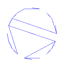
And here is an example of random tree:

> plotTree(draw([T,tbf],size=20));

>

Forests

In order to dissociate the trees in a forest, let us substitute to each vertex of a tree another vertex together with a forest

> fo:={B=Prod(Sequence(B),V,Sequence(B)),
V=Union(Prod(Z, F)),
F=Union(Epsilon, Prod(V, Sequence(B)))};

> seq(count([F, fo], size=i), i=1..10);

Connected and general graphs

Connected graphs

To see how nc-graphs are built, consider the set of childs attached to the root . The graphs built on and are connected by hypothesis, while between any two other vertices and one can have either one connected graph or two connected graphs.

But any graph built from a sequence of successive vertices of the circle is a system of arches since the arcs which are chords are not allowed to cross. The endpoints of these arches are shared by the graphs built to the left and to the right of a given , so that we shall say that the size of an arch built on points is . At last, we are interested here in Elementary Arches, that is arches that always contain an arc between the firt and last points. General arches are easily obtained by sequencing EAs.

From this discussion we derive the Combstruct specification of NC graphs containing at least 2 vertices. In particular, the 5 arguments of a C entity are as follows:

1.first Z: the root of the graph

2.second Z: the lefmost point of the first EA

3 and 4. the two EAs built on and

5.the sequence of EAs found between two consecutive childs of . The first term corresponds to one EA,

and the second one to two EAs. For the latter case, the Z in the Prod stands for the lefmost point of the secong EA.

> ar:={EA = Union(Sequence(EA, card >= 2),
Prod(Z, Sequence(EA), Sequence(EA))
),
C=Union(Z,
Prod(Z,Z,Sequence(EA), Sequence(EA),
Sequence(Union(Sequence(EA,card>=1), Prod(Z,Sequence(EA),Sequence(EA))))))};

We can now count the number of elementary arches of a given size. The sequence found is not in [Sloa95]:

> seq(count([EA,ar], size=i),i=1..20);

> allstructs([EA,ar],size=2);

We can also count the number of NC-graphs. The corresponding sequence turns out to be M3594 in [Sloa95] and gives the reverse

of the g.f. for squares:

> seq(count([C,ar], size=i),i=1..10);

As usual, we can get all the structures of a given size, or just draw some of them:

> allstructs([C,ar],size=3);

> draw([EA,ar],size=10);

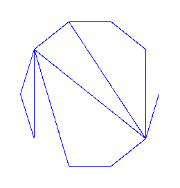
And an example of random graph:

> plotNCGraph(draw([C,ar],size=10));

>

General graphs

As observed in [FlaNo97], a general graph is obtained from a connected one by the substitution Z -> Prod(Z, G). So that we just have to rewrite the previous grammar by adding a new symbol which makes this substitution. Notice however that the decomposition of a connected graph misses a configuration for general graphs: the one where vertex does not have any child, which we therefore add:

> br:={EA = Union(Sequence(EA, card >= 2),
Prod(V, Sequence(EA), Sequence(EA))
),
V=Union(Prod(Z, G)),
G=Union(Epsilon,
Prod(Z, G),
Prod(V,V,Sequence(EA), Sequence(EA),
Sequence(Union(Sequence(EA,card>=1), Prod(V,Sequence(EA),Sequence(EA)))))
)
};

The number of graphs is given by the following sequence, not to be found in [Sloa95]:

> ggSeq:=[seq(count([G, br], size=i), i=0..20)];

In this case, it also turns out that the differential equation verified by is of order 1:

> ggDiffEq:=listtodiffeq(ggSeq,y(x));

From this equation and the condition , we get the following closed form:

> closedForm:=dsolve(ggDiffEq[1],y(x));
subs(_C1=-1/2,closedForm);

As shown in [FlaNo97], this corresponds to the general term:

> cn:=proc(n)
local k,l;
sum((-1)^k*product(2*l-1,l=1..n-k-1)/(factorial(k)*factorial(n-2*k))*3^(n-2*k)*2^(-k-2), k=0..iquo(n,2))
end:

> gn:=proc(n) 2^n*cn(n-1) end;

> seq(gn(i), i=3..10);

Dissections and partitions

Dissections

A dissection of a convex polygon is a partition of the polygon into polygonal regions by means of non-crossing diagonals. If the polygonal region containing the edge has sides, one gets a bigger dissection by replacing the edges by a dissection. So that a dissection is either an edge connecting two vertices or a sequence of dissections. The tricky point in sequencing 2 dissections consists in not counting the same vertex twice, as for the connected graphs above. When sequencing dissections, we therefore assume that each dissection provides its rightmost point while the lefmost one is the rightmost point of the dissection to the left in the sequence. With this convention, the number of dissections of size actually counts the number of dissections of a polygon with vertices, and the grammar is:

> dissG:={Di=Union(Z, Sequence(Di, card >= 2))};

The corresponding sequence, M2898 in [Sloa95] and related to Schroeder's second problem is:

> seq(count([Di, dissG], size=i), i=1..10);

Partitions

A non-crossing partition of size is a partition of [n]={1,2,...,n} such that if a<b<c<d and a block contains and , then no block contains and . Given a partition block, possibly empty, one gets a bigger partition by subsituting to each vertex the product between Z and another partition. So that:

> partG:={P=Sequence(V), V = Prod(Z,P)};

We get the sequence of Catalan numbers, which can be checked in terms of generating functions:

> seq(count([P, partG], size=i), i=1..10);

> gfsolve(partG, unlabelled, z);

Univariate asymptotics

Asymptotic counting: algorithm

Outline

As shown in [FlaNo97] for the six NC configurations we are interested in, the generating function satisfies an algebraic equation. In the case of NC forests for example, we have:

> eq:=y^3+(-z+z^2-3)*y^2+(z+3)*y-1;

Like in many implicitely defined functions [Dr97, HaPa73], we expect a priori to have locally an expansion of the square-root type, that is:

By a singularity analysis at the dominant singularity and denoting , we get:

or

We now examplify this method for the class of NC-forests. The singulatities sought may arise at those points such that E(z,y)=0 and . In order to get the candidates satisfyning these conditions, we just have to eliminate between the two previous equations through a resultant computation:

> res_y:=resultant(eq,diff(eq,y),y);
res_y:=expand(normal(res_y/gcd(res_y,diff(res_y,z))));
Omega[0]:=normal(res_y/z^ldegree(res_y));

And the singularities sought are the solutions of the previous equation whose modulus is smaller than 1. If the set found has cardinality one, we are done. It actually turns out that this is the case for all our configurations but the connected graphs where a `ghost' singularity has to be elimanated by an external argument --see [FlaNo97]. In our case:

> rhonums:=[fsolve(Omega[0],z,complex)];
Omega[1]:=map(proc(x) if abs(x)<1 then x fi end,rhonums);

And a convenient way to represent our singularity both in symbolic and numerical form is:

> rho_symb:=RootOf(Omega[0], z, op(Omega[1]));

Since in our case the dominant coefficient of the equation in does not vanish, the function remains finite at its singularity. Its value is also the quantity defined above. Since the point is a singularity, we have and . Candidate values for are therefore obtained as follows:

> deq:=subs(z=rho_symb, diff(eq,y));
print(`Candidate values for function at singularity`);
tau_vals:=[fsolve(deq,y)];
print(tau_vals);

Plugging back these candidates into the equation eq, we could get the correct one from a carefully controlled numerical analysis:

> eTau:=subs(z=rho_symb, eq);
[seq( evalf(subs(y=tau_vals[i], eTau)), i=1..nops(tau_vals))];

To get the constant we are missing, let us just compute the Puiseux expansions verified by with the algeqtoseries procedure from the gfun package:

> all_puis:=algeqtoseries(subs(z=rho_symb*(1-t^2),eq),t,y,6);

and select those with a term --which corresponds to the square-root sought due to the change of variable :

> #--convert into series i.e. remove the O()
all_puis_s:=map(eval, map2(subs, O=0, all_puis));
#--collect the coeff in t and select the non-null one(s)
c1:=map(proc(x) if x<>0 then x fi end, map(coeff, all_puis_s, t, 1));
print(`Constant`, evalf(c1,10));

Should we have found several expansions containing a term, the right one could have been selected from the formula and . Also note that the minus sign has to be adopted for since the generating function increases with its argument.

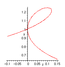
We can locally plot the algebraic curve in the neighborhood of the singularity:

> implicitplot(eq, z=-.1..0.15, y=-1..1.3, numpoints=5000);

Putting everything together, we get the following procedure which we apply to the remaining NC configurations.

Implementation

We first look for the singularity(ies) of smallest modulus(i):

> locateDominantSing := proc(eq, y, z)
local res_y, Omega, rhonums,
rho_symb;

#--we look for the z such that eq and diff(eq,y) have a common root y
res_y:=resultant(eq,diff(eq,y),y);
res_y:=expand(normal(res_y/gcd(res_y,diff(res_y,z))));
Omega[0]:=normal(res_y/z^ldegree(res1_y));
rhonums:=[fsolve(Omega[0],z,complex)];

#--we are just interested in roots of modulus < 1
Omega[1]:=map(proc(x) if abs(x)<1 then x fi end,rhonums);
if nops(Omega[1])<>1 then
ERROR(`More than one root of modulus < 1: not implemented!`) fi;

rho_symb:=RootOf(Omega[0], z, op(Omega[1]));
print(`Singularity is`); print(rho_symb);

rho_symb
end:

And then the asymptotic expansion. The values returned are:
1.the symbolic expressions for the constant
2.the dominant singularity
3.the Puiseux expansion

> singExpansion:=proc(eq, y, z)
local rho_symb,
deq, tau_vals,
all_puis, all_puis_s, c1;

#--numerical and symbolic representation of the singularities
rho_symb:=locateDominantSing(eq, y, z);

#--values of the function at the singularity
deq:=subs(z=rho_symb, diff(eq,y));
print(`Candidate values for function at singularity`);
tau_vals:=[fsolve(deq,y)];
print(tau_vals);

#--Puiseux expansion; we expect a single exp. to have a t term
all_puis:=algeqtoseries(subs(z=rho_symb*(1-t^2),eq),t,y,6);

#--convert into series i.e. remove the O()
all_puis_s:=map(eval, map2(subs, O=0, all_puis));
#--collect the coeff in t and select the non-null one(s)
c1:=map(proc(x) if x<>0 then x fi end, map(coeff, all_puis_s, t, 1));

if nops(c1)<>1 then
print(`Problem in singular expansion`); print(all_puis); RETURN(FAIL)
else
c1:=op(c1); if evalf(c1)>0 then c1:=-c1 fi
fi;

#--returns the constant c1 and the singularity in symbolic forms
print(`c1 constant`, c1,evalf(c1,20));
[c1,rho_symb, my_puis]
end:

Applications to non-crossing configurations

We now present the whole chain that goes from the grammars specification to the asymptotic machinery. More precisely, for each of the NC configurations studied above, we:

1.call Combstruct[gfeqns] to retrieve the system of equations verified by the generating functions associated with the grammar,

2.compute the algebraic equation verified by a given generating function with gfun[algfuntoalgeq],

3.feed this equation to the asymptotic machinery developped above.

Trees

Generating functions associated with the grammar:

> gfeqns(tbf, unlabelled, z);

> treesSys:=gfsolve(tbf, unlabelled, z);

Algebraic equation:

> trees:=algfuntoalgeq(subs(treesSys,T(z)), y(z));

Asymptotic machinery:

> resTrees:=singExpansion(trees, y, z):

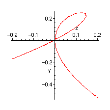
Plot of the singularity:

> implicitplot(trees, z=-0.2..0.2, y=-1..1, numpoints=5000);

Forests

> forests:=y^3+(-z+z^2-3)*y^2+(z+3)*y-1;

> resForests:=singExpansion(forests, y, z):

Connected graphs

Generating functions associated with the grammar:

> CGSys:=gfsolve(ar, unlabelled, z);

Algebraic equation:

> CG:=algfuntoalgeq(subs(CGSys,C(z)), y(z));

Asymptotic machinery:

> resCG:=singExpansion(CG, y, z):

Error, (in locateDominantSing) More than one root of modulus < 1: not implemented!

As observed in [FlaNo97], due to the two singularities found, we need additional information to select the right one. Eliminating the negative value and performing the previous computations yields the following and :

> resCG[1]:=-RootOf(54*_Z^2-7+72*RootOf(-1+108*_Z^2,.96225044864937627418e-1));

> resCG[2]:=RootOf(-1+108*_Z^2,.96225044864937627418e-1);

Plot of the singularity:

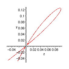
> implicitplot(CG, z=-0.05..0.15, y=-.05..0.2, numpoints=10000);

General graphs

Generating functions associated with the grammar:

> GGSys:=gfsolve(br, unlabelled, z);

Algebraic equation:

> GG:=algfuntoalgeq(subs(GGSys,G(z)), y(z));

Asymptotic machinery:

> resGG:=singExpansion(GG, y, z):

Plot of the singularity:

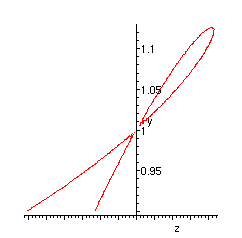
> implicitplot(GG, z=-0.2..0.1, y=0.9..1.2, numpoints=10000);

Dissections

> dissSys:=gfsolve(dissG, unlabelled, z);

> diss:=algfuntoalgeq(subs(dissSys,Di(z)), y(z));

> resDiss:=singExpansion(diss, y, z):

It should be noticed that the equation obtained in the paper and stated below in slightly different.But remember that counts here the number of dissections of a polygon with vertices. Of course, we still have the same singularity:

> diss2:=2*y^2-z*(1+z)*y+z^3:

> resDiss2:=singExpansion(diss2, y, z):

Plot of the singularity:

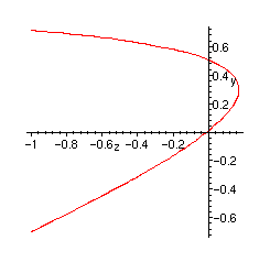
> implicitplot(diss, z=-1..1, y=-1..1, numpoints=1000);

Partitions

> partsSys:=gfsolve(partG, unlabelled, z);

> parts:=algfuntoalgeq(subs(partsSys,P(z)), y(z));

> resParts:=singExpansion(parts, y, z);

Here we are in trouble since there are 2 Puiseux expansions with terms. But only the first one makes sense since the generating function increases with its argument. So that:

> resParts[1]:=2: resParts[2]:=1/4:

Plot of the singularity:

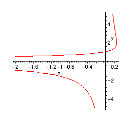
> implicitplot(parts, z=-2..1, y=-5..5, numpoints=1000);

Exact and estimated values: comparisons

We have already seen that an estimate of the number of objects of size is given by:

> nbEnt:=proc(c1,rho, n)
evalf(c1*rho^(-n)/(2*sqrt(Pi*n^3)))
end;

Comparisons with the exact values are as follows. It is interesting to observe that these values are within about 2% in any case:

Trees

> exactTr:=evalf(count([T,tbf], size=100));

> estimTr:=nbEnt(resTrees[1],resTrees[2],100);

> exactTr/estimTr;

Forests

> exactFo:=evalf(count([F,fo], size=100));

> estimFo:=nbEnt(resForests[1], resForests[2], 100);

> exactFo/estimFo;

Connected graphs

> exactCo:=evalf(count([C,ar],size=100));

> estimCo:=nbEnt(resCG[1],resCG[2],100);

> exactCo/estimCo;

General graphs

> exactGG:=evalf(count([G, br], size=100));

> estimGG:=nbEnt(resGG[1], resGG[2], 100);

> exactGG/estimGG;

Dissections

> exactDiss:=evalf(count([Di, dissG], size=100));

> estimDiss:=nbEnt(resDiss[1], resDiss[2], 100);

> exactDiss/estimDiss;

Partitions

> exactPart:=evalf(count([P, partG], size=100));

> estimPart:=nbEnt(resParts[1], resParts[2], 100);

> exactPart/estimPart;

>

References

[Dr97] M. Drmota, Systems of functional equations, Random Structures and Algorithms 10, 1-2, 1997.

[FlaNo97] P. Flajolet and M. Noy, Analytic Combinatorics of Non-Crossing Configurations, Rapport de Recherche INRIA No. 3196, 1997.

[HaPa73] F. Harary and E.M. Palmer, Graphical Enumeration, Academic Press, 1973.

[Sloa95] N.J.A. Sloane and S. Plouffe, The Encyclopedia of Integer Sequences, Academic Press, 1995.