Monomer-Dimer Tilings

F. Cazals, December 1997.

A fundamental problem in lattice statistics is the monomer-dimer problem, in which the sites of a regular lattice are covered by non-overlapping monomers and dimers, that is squares and pairs of neighbor squares. An example of such a tiling for a chessboard with and is depicted below. The relative number of monomers and dimers can be arbitrary or may be constrained to some density , and the problem can be generalized to any fixed dimension . This model was introduced long ago to investigate the properties of adsorbed diatomic molecules on a crystal surface [Rob35], and its three-dimensional version occurs in the theory of mixtures of molecules of different sizes [Gug52] as well as the cell cluster theory of the liquid state [CoAl55]. Practically, most of the thermodynamic properties of these physical systems can be derived from the number of ways a given lattice can be covered, so that a considerable attention has been devoted to this counting question. For any fixed dimension and any monomer density , a provably good polynomial time approximation algorithm is exposed in [KenAl95]. But exact counting results are still unknown even in dimension two.

The goal of this worksheet is to show that these questions are amenable to an automated computer algebra treatment which goes from the specifications of the coverings constructions in terms of Combstruct grammars, to the asymptotics using rational generating functions and the numeric-symbolic method exposed in [GoSa96]. In particular we shall be interested in enumerating the tilings for a vertical strip of constant width in terms of multivariate rational generating functions, from which the average number of pieces or the expected proportions of the three types of pieces in a random tiling are easily derived.

This will also enable us to establish a provably good sequence of upper and lower bounds for the connectivity constant where counts the number of ways to tile an cheesboard.

But before getting started, we need to load the Combstruct library, as well as the piece of code doing the asymptotics of rational fractions:

> with(combstruct): with(gfun): read `ratasympt.mpl`;read `./gfsolve.mpl`;

References

[CoAl55] E.G.D. Cohen et al., A cell-cluster theory for the liquid state II, Physica XXI, 1955.

[Fin97]S. Finch, Favorite Mathematical Constants, http://www.mathsoft.com/cgi-shl/constant.bat.
[GoSa96] X. Gourdon and B. Salvy, Effective Asymptotics of linear recurrences with rational coefficients, Discrete Mathematics, Vol. 153, 1996.

[Gug52] E.A. Guggenheim, Mixtures, Clarendon Press, 1952.
[Ken95] C. Kenyon et al., Approximating the number of Monomer-Dimer Coverings of a Lattice, Proc. of the 25th ACM STOC, 1993.
[Rob35]J.K. Robert, Some properties of adsorbed films of oxygen on tungsten, Proc. of the Royal Society of London, Vol. A 152, 1935.

[Sloa95] N.J.A. Sloane and S. Plouffe, The Encyclopedia of Integer Sequences, Academic Press, 1995.

A step-by-step example

We first observe that the number counting the different tilings of a vertical slice of width 1 has a well known expression: since height can be reached from height by adding a monomer and from height with a vertical dimer, we have with , that is the Fibonacci recurrence. This can be checked directly with Combstruct:

> TGr:={T=Sequence(Union(monomer,dimer)),monomer=Z,dimer=Prod(Z,Z)};

And we can retrieve the corresponding rational Generating Function with gfsolve:

> gfsolve(TGr,unlabelled, z);

More interesting is the case m=2 which we examine examine now.

Tiling a slice of width

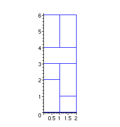
An example covering of a 2x6 lattice is depicted below. If we draw a horizontal line at height 0, it turns out that we do not `cut' any piece, which we encode by MM. At height 1, we cut the lefmost vertical dimer but just touch the monomer topmost side, which we encode by PM. At height 2 the leftmost P turned into an M since we now touch the dimer boundary, while on the right side we added a dimer and have a P. More generally, we shall assign to each height of the construction containing a monomer or dimer boundary a word of length on the alphabet as follows: the th digit of the word is if an horizontal line at this particular height splits a vertical domino located in the th column, and otherwise. To summarize our example we therefore have MM, PM, MP, MM, MM,MM at the heights 0,1,2,3,4,6. (BTW, M stands for Minus and P for Plus!)

This encoding is not one-to-one since whenever we find two consecutive Ms, we do not know wether they are on top of two monomers or of a horizontal dimer. But it is sufficient to incrementally build all the possible configurations by recording the status of the fringe. If , the possible fringes are MM,MP,PM and each of them can be derived from a combination of the others and of monomers and dimers. For example, the configuration MM can be reached in 5 different ways by:

-stacking a horizontal dimer H, two monomers C,C, or two vertical dimers V,V on top of a MM configuration,

-adding a monomer C to the right column of a PM configuration or to the left one of a MP.

The remaining transitions follow similar rules. And in order to characterize the ordinate reached by the construction, we can mark the height reached by the bottommost piece whose elevation gain is 1 or 2 at each step of the construction. Putting everything together and associating the symbols and to the number of horizontal dimers, vertical dimers, monomers and the height yields the following Combstruct grammar:

> Gr2:={MM=Union(Epsilon,Prod(S, MM, H), Prod(S, MM, C,C),
Prod(S,PM, C),Prod(S,MP, C),Prod(S,S,MM,V,V)),
PM=Union(Prod(S,MM, V, C), Prod(S,MP,V)),
MP=Union(Prod(S,MM, C, V), Prod(S,PM,V)),
H=Epsilon,V=Epsilon,C=Epsilon,S=Atom}:

The ordinary generating functions can be derived by Combstruct[gfsolve]:

> GF2Sys:=gfsolve(Gr2, unlabelled, z, [[h,H], [v,V], [c,C]]);

Furthermore we can isolate the GF corresponding to the MM fringes; the coefficient of in this GF counts the number of ways to tile a chessboard with respectively and horizontal and vertical dimers and monomers:

> GF2:=subs(GF2Sys,MM(z,h,v,c));

The number of configurations up to a given height independently of the number and kind of pieces used can be retrieved by erasing the dimers and monomers markers followed by a Taylor expansion:

> GF2h:=subs([h=1,v=1,c=1],GF2);series(GF2h,z=0,11);

This sequence does not appear in [Sloa95]. It can be checked that these values match those computed directly from the grammer by Combstruct[count]:

> seq(count([MM,Gr2], size=i), i=0..10);

Another way to compute the exact number of tilings for large values of is through the recurrence equation satisfied by the Taylor coefficients and computed by gfun[diffeqtorec]:

> diffeqtorec(y(z)-GF2h,y(z),u(n));

> p2:=rectoproc(",u(n)):

> for i from 1 to 10 do i,p2(i) od;

For example:

> p2(1000);evalf(");

But as we shall see now, asymptotic estimates can be derived much faster.

Asymptotic estimates of the number of tilings

We have just seen that the number of configurations is encoded by the rational generating function GF2h(z). An elegant way to access its Taylor coefficients is therefore through a full partial fraction decomposition yielding linear denominators:

> fpf:=convert(GF2h,fullparfrac,z);

The term in comes from the contributions of the roots of in the expansion of

> el:=op(1,fpf);

and since there are 3 singularities, the main asymptotic contribution comes from the one with smallest modulus:

> fsolve(-3*_Z+1+_Z^3-_Z^2,_Z);

> root1:=RootOf(-3*_Z+1+_Z^3-_Z^2,.3111078175);
root2:=RootOf(-3*_Z+1+_Z^3-_Z^2,-1.481194304);
root3:=RootOf(-3*_Z+1+_Z^3-_Z^2,2.170086487);

On this example the dominant pole is clearly so that the main contribution is encoded by:

> el1:=subs(_alpha=root1,el);

> evalf(");

Extracting the term in in the previous expression produces the estimate:

> es2:=n->.2067595751*(1/.3111078175)^(n+1);

> seq(es2(i),i=1..10);

To sum up, from the rational generating function we have:

-performed a full partial fraction decomposition,

-computed the singularities and sorted them by increasing moduli,

-extracted the contribution of the singularity with smallest modulus.

The key step consists in deciding which are the singularity (ies) with smallest modulus (i), and can be performed numerically using properties of polynomials with integer coefficients --see [GoSa96]. This is implemented by the ratasympt function --whose optional th argument corresponds to the number of singularity layers the user wants to take into account. In particular to retrieve the main contribution, one writes:

> layer1:=ratasympt(GF2h,z,n,1);nbCfs1:=evalf(layer1);

And to take into account all the layers:

> layers:=ratasympt(GF2h,z,n);nbCfs:=evalf(layers);

We can check that the second approximation is more accurate:

> evalf(seq(subs(n=i, layer1), i=1..10));

> evalf(seq(subs(n=i, layers), i=1..10));

> seq(p2(i),i=1..10);

The proportion of monomers and dimers

We now address the computation of the average number of pieces in a random tiling. From the multivariate generating function we can merge the three types of pieces as follows:

> GF2;stij:=subs([h=t,v=t,c=t], GF2);

The coefficient of in counts the number of tilings at height with exactly pieces of any type. To get the total number of pieces we just have to compute the derivative with respect to and substitute :

> sstij:=subs(t=1, diff(stij,t));

For example, the total number of dimers and monomers used in all the configurations tilling the square is 20:

> series(",z=0,5);

As before, we can compute an estimate of the total number of pieces in all the configurations at a given height:

> ratasympt(sstij,z,n,1);

> nBDPiecesN:=evalf(");

So that the average number of pieces is asymptotically equivalent to:

> avNbD:=expand(nBDPiecesN/nbCfs1);

And the average number of pieces per layer in a tiling of height is therefore:

> asympt("/n,n);

The number of occurrences and the proportions of dimers and monomers can be computed in the same way by erasing the irrelevant indeterminates:

> pieceProportion:=proc(MGF, keptPiece)
local forSubs, stij, sstij, nbp;

forSubs:={h=1,v=1,c=1} minus {keptPiece=1};
stij:=subs([op(forSubs)], MGF);
sstij:=subs(keptPiece=1, diff(stij,keptPiece));
nbp:=evalf(ratasympt(sstij,z,n,1));
asympt(nbp/nBDPiecesN,n,2)
end:

And we end up with:

> nbh:=pieceProportion(GF2,h);
nbv:=pieceProportion(GF2,v);
nbc:=pieceProportion(GF2,c);

Plotting routines archive

The figures above were plotted with the following functions:

> dominoH:=proc(x,y) [[x,y], [x+2,y], [x+2,y+1], [x,y+1], [x,y]] end:
dominoV:=proc(x,y) [[x,y], [x+1,y], [x+1,y+2], [x,y+2], [x,y]] end:
dominoC:=proc(x,y) [[x,y], [x+1,y], [x+1,y+1], [x,y+1], [x,y]] end:

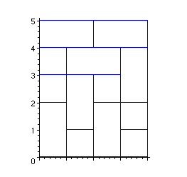
> plot([dominoV(0,0), dominoC(0,2),dominoC(0,3),
dominoC(1,0),dominoV(1,1),dominoH(1,3),
dominoV(2,0),dominoC(2,2),
dominoC(3,0),dominoC(3,1),dominoV(3,2),
dominoH(0,4),dominoH(2,4)],scaling=constrained,color=blue);

>

> plot([dominoV(0,0), dominoC(1,0),dominoV(1,1),dominoC(0,2),dominoH(0,3),dominoV(0,4),dominoV(1,4)], scaling=constrained,color=blue);

Automatic counting in a slice of width

Computing the generating functions

We now show how to automate the previous computations for any integer . The first task consists in generating the words on the binary alphabet , and this is easily done with a Combstruct grammar as follows:

> allMPWords:=proc(m::integer)
local i, MPGr, mps1, mps2, Pm;

MPGr:={AllMP=Sequence(MP), MP=Union(M,P), M=Atom, P=Atom};
mps1:=allstructs([AllMP, MPGr], size=m);
mps2:=convert(map(proc(x) cat(op(x)) end, mps1), set);
Pm:=cat(seq(P,i=1..m));
[op(mps2 minus {Pm})]
end:

For example if :

> allMPWords(3);

More interesting is the generation of the transitions between these words. Let be one of them and suppose we want to figure out all the fringes can be derived from. Suppose for example the th letter of is a ; this means that the th letter of the fringe was derived from was and that a vertical dimer was put on top of this . Similar rules applies if the th digit is a . And since the letter of a given fringe are independent --except for two consecutive s that may come from an horizontal dimer, it suffices to recursively examine the digits from left to right as follows:

> #--pattern is the fringe to be built, e.g. MMPMM
recComesFrom:=proc(pattern::string, idx::integer, prefix::string, mul::list, result::table)
local prodRes, m, Mm, Pm;

if (idx>length(pattern)) then #--stores the result into an indexed table
prodRes:=Prod(S,prefix, op(mul));
if not assigned(result[pattern]) then result[pattern]:={prodRes}
else result[pattern]:=result[pattern] union {prodRes}
fi
else
#--we examine the idx^{th} letter of the target
if substring(pattern,idx)=P then
recComesFrom(pattern, idx+1, cat(prefix,M), [op(mul), V], result)
else #target=M
recComesFrom(pattern, idx+1, cat(prefix,P), mul, result);
recComesFrom(pattern, idx+1, cat(prefix,M), [op(mul), C], result);

#--we may have MM=Prod(MM,H)
if (length(pattern)>idx) and (substring(pattern,idx+1)=M) then
recComesFrom(pattern, idx+2, cat(prefix,M,M), [op(mul), H], result)
fi
fi
fi;

#--some extra work for M^m
m:=length(pattern);
Mm:=cat(seq(M,i=1..m));
if pattern=Mm then
Pm:=cat(seq(P,i=1..m));
result[Mm]:=result[Mm] minus {Prod(S,Pm)}
union {Epsilon,Prod(S,S,Mm,seq(V,i=1..m))}
fi
end:

Here is the table for :

> table3:=table():for i in allMPWords(3) do recComesFrom(i, 1, ``, [], table3) od:print(table3);

The tables entries are merged as follows:

> setGrammarFromTable:=proc(aTable)
local aList, transitions, x;
aList:=op(op(aTable));#--[a={Prod(...), Prod(...)}, ...]
transitions:=seq(op(1,x)=Union(op(op(2,x))), x=aList);
{transitions} union {H=Epsilon,V=Epsilon,C=Epsilon,S=Atom}
end:

This yields the grammar:

> Gr3:=setGrammarFromTable(table3);

This is solved as usual:

> MM3GFSys:=gfsolve(Gr3, unlabelled, z, [[h,H], [v,V], [c,C]]);
MM3GF:=subs(MM3GFSys,MMM(z,h,v,c));

Putting everything together, we end up with a procedure which takes as entry and returns the grammar:

> getGrammar:=proc(m::integer)
local i, MPTable;

MPTable:=table();
for i in allMPWords(m) do recComesFrom(i,1,``,[],MPTable) od;
setGrammarFromTable(MPTable)
end:

getMmGFun:=proc(m::integer)
local i, MPTable,Grm,MMmGFSys;

Grm:=getGrammar(m);
MMmGFSys:=gfsolve(Grm, unlabelled, z, [[h,H], [v,V], [c,C]]);
subs(MMmGFSys,cat(seq(M,i=1..m))(z,h,v,c));
end:

The computation to be carried out being quite heavy for 4-variate generating functions, we can alleviate it be keeping only the markers for the total number of pieces and the height:

> getMmGFunZ:=proc(m::integer)
local i, MPTable,Grm,GrmM,MMmGFSys;

MPTable:=table();
for i in allMPWords(m) do recComesFrom(i,1,``,[],MPTable) od;
Grm:=setGrammarFromTable(MPTable);
MMmGFSys:=gfsolve(Grm, unlabelled, z);
subs(MMmGFSys,cat(seq(M,i=1..m))(z));
end:

Asymptotics

We can now compute the generating functions for small values of :

> gf:='gf':

> for i from 1 to 5 do i,time(assign(gf[i],getMmGFunZ(i))),gf[i] od;

For bigger ones, the grammar size, that is , inherently yields a linear system with large coefficients whose resolution is very much time consuming. So that for , a better alternative to running getMmGFunZ(m) is to retrieve the result in the archive below!

From these generating functions we can easily isolate the main contribution to the asymptotic equivalent with the ratasympt procedure:

> asGf:='asGf':

> for i from 1 to 6 do assign(asGf[i],ratasympt(gf[i],z,n,1)),evalf(asGf[i]) od;

It should be observed that these estimates correspond to huge expressions. For for example:

> asGf[5];

As observed in [Fin97], if denotes the number of tilings of a chessboard, an interesting value for the physical applications is .

No exact expression for this limit is known, although the approximation 1.940215531 is generally agreed on. The first terms of the sequence can be computed from the previous approximations and are consistent with 1.94:

> nn:='nn':

> for i from 1 to 6 do assign(nn[i],coeff(series(gf[i],z=0,i+1),z,i)),evalf((nn[i])^(1/(i*i))) od;

But more interesting is the following observation. Suppose for example is a multiple of 6. To tile a chessboard we can put side by side slices of width 6. In this case with the singularity of smallest modulus of the denominator of . If is not a multiple of 6, it suffices to complete with at most 5 vertical stripes of width 1, but this does not change the limit. The interest in using as many slices of maximal width is to minimize the number of joints where the overlaps are not taken into account. The sequence therefore provides lower bounds for the constant . An upper bound can be obtained in the same way by having slices of width 6 overlap on a position, and the corresponding sequence is .

> for i from 2 to 6 do i,(1/op(1,denom(evalf(asGf[i]))))^(1./i),(1/op(1,denom(evalf(asGf[i]))))^(1./(i-1)) od;

At last a trick we can use to try to guess the value of is Romberg's convergence acceleration. Let be a sequence known to converge to . If the rate of convergence is of the form , then is . On our example, although the upper bound does not make sense due to too erroneous initial values, after a single step the lower bound gets close to the commonly accepted value:

> u[2]:=1.792852404:u[4]:=1.863497010:
v[2]:=3.214319743:v[4]:=2.293180643:
2*u[4]-u[2],2*v[4]-v[2];


u[3]:=1.838281935:u[6]:=1.888704987:
v[3]:=2.492402505:v[6]:=2.144850135:
2*u[6]-u[3],2*v[6]-v[3];

Generating functions archive

> gf[1]:=-1/(-1+z^2+z);

> gf[2]:=-1/(-3*z+1-z^2+z^3)*(z-1);

> gf[3]:=-(z^4+z^3-4*z^2-z+1)/(14*z^2-1+4*z+z^6-10*z^4);

> gf[4]:=-(1-4*z-15*z^2+20*z^3+z^7-11*z^5-2*z^6+10*z^4)/(z^9-z^8-23*z^7+29*z^6+91*z^5-111*z^4-41*z^3+41*z^2+9*z-1);

> gf[5]:=-(z^18+2*z^17-45*z^16-68*z^15+654*z^14+870*z^13-3820*z^12-4700*z^11+9255*z^10+9448*z^9-11175*z^8-7532*z^7+6956*z^6+1994*z^5-1794*z^4-88*z^3+113*z^2+6*z-1)/(z^20+2*z^19-65*z^18-140*z^17+1281*z^16+2538*z^15-10366*z^14-17604*z^13+38553*z^12+50158*z^11-73623*z^10-60482*z^9+74665*z^8+26564*z^7-35106*z^6-898*z^5+4757*z^4+16*z^3-229*z^2-14*z+1);

> gf[6]:=-(-1+311*z^2-3891*z^3-12057*z^4-315889*z^6-2997721*z^7+218447*z^5+13467571*z^9+8754480*z^8+23*z-458919487*z^18-303976032*z^17+612805499*z^16+207743591*z^15-496137395*z^14-56233657*z^13+240612231*z^12-14684235*z^11-66016499*z^10+206819317*z^20+249194245*z^19-109*z^32-36273*z^29+861*z^31+7443809*z^24+37223601*z^23-123372421*z^21-54160427*z^22-6708699*z^25+z^34-29377*z^28+686517*z^27-338040*z^26+3521*z^30-7*z^33)/(1-576*z^2+6080*z^3+42422*z^4-443404*z^6+12931566*z^7-453004*z^5-83558644*z^9-25517604*z^8-36*z+4169343006*z^18+2978277152*z^17-4669345206*z^16-1630080704*z^15+3235975264*z^14+274712602*z^13-1335612340*z^12+154307596*z^11+295510396*z^10-2310327672*z^20-2919950172*z^19+5736*z^32+1503868*z^29-62874*z^31-149620588*z^24-626694028*z^23+1717916424*z^21+777289050*z^22+141424642*z^25-8*z^35-138*z^34+z^36-94620*z^28-19237868*z^27+13835164*z^26-81796*z^30+1224*z^33);

>

>

>

Conclusion

We showed that various parameters related to dimer-monomer tilings such as the average number of pieces or the relative numbers of horizontal dimers and monomers in a random tiling of height in a strip of width can be computed very easily using Combstruct and ratasympt. More precisely Combstruct is used to define the grammars the tilings are derived from, and ratasympt is used to perform asymptotic expansions on rational fractions with rational coeficients.

About the number of different tilings of a chessboard, altough the method presented here is limited due to the exponential growth of the grammar describing these tilings, the very first terms computed provide provably good upper and lower bounds for the connectivity constant . More precisely:

Theorem . The connectvity constant for two dimensional monomer-dimer tilings satisfies

and